Cleaning and structuring information in textual data

If you want to try the examples in this tutorial:

1 Introduction

1.1 Recap

As mentioned in the introduction to this section on natural language processing, the main goal of the techniques we will explore is the synthetic representation of language.

Natural Language Processing (NLP) aims to extract information from text through statistical content analysis. This definition includes a wide range of NLP applications (translation, sentiment analysis, recommendation, monitoring, etc.).

This approach involves transforming a text—understandable by humans—into a number, which is the appropriate format for a computer in the context of statistical or algorithmic approaches.

Turning textual information into numerical values suitable for statistical analysis is no easy task. Text data are unstructured since the sought-after information—specific to each analysis—is hidden in a large mass of information that must also be interpreted within a certain context (the same word or phrase can have different meanings depending on the context).

If that wasn’t already difficult enough, there are additional challenges specific to text analysis, as this data is:

• noisy: spelling, typos…
• evolving: language changes with new words, meanings…
• complex: variable structures, agreements…
• ambiguous: synonymy, polysemy, hidden meanings…
• language-specific: no single set of rules applies across languages
• high-dimensional: infinite combinations of word sequences

1.2 Chapter Objective

In this chapter, we will focus on frequency-based methods within the bag of words paradigm. These are somewhat old school compared to the more sophisticated approaches we’ll cover later. However, introducing them allows us to address several typical challenges of text data that remain central in modern NLP.

The main takeaway from this section is that since text data is very high-dimensional—language is a rich object—we need methods to reduce the noise in our text corpora to better capture the signal.

This part serves as an introduction, drawing on classic works of French and English literature. It will also present some key libraries that form part of the essential toolkit for data scientists: NLTK and SpaCy. The following chapters will then focus on language modeling.

The SpaCy Library

NLTK is the historical text analysis library in Python, dating back to the 1990s. The industrial application of NLP in the world of data science is more recent and owes a lot to the increased collection of unstructured data by social networks. This has led to a renewal of the NLP field, both in research and in its industrial application.

The spaCy package is one of the tools that enabled this industrialization of NLP methods. Designed around the concept of data pipelines, it is much more convenient to use for a text data processing chain that involves multiple transformation steps.

1.3 Method

Text analysis aims to transform text into manipulable numerical data. To do this, it is necessary to define a minimal semantic unit. This textual unit can be a word, a sequence of n words (an ngram), or even a string of characters (e.g., punctuation can be meaningful). This is called a token.

Various techniques (such as clustering or supervised classification) can then be used depending on the objective, in order to exploit the transformed information. However, text cleaning steps are essential. Otherwise, an algorithm will be unable to detect meaningful information in the infinite range of possibilities.

The following packages will be useful throughout this chapter:

!pip install pywaffle
!pip install spacy
!pip install plotnine
!pip install great_tables
!pip install wordcloud

2 Example Dataset

2.1 The Count of Monte Cristo

The example dataset is The Count of Monte Cristo by Alexandre Dumas. It is available for free on the http://www.gutenberg.org (Project Gutenberg) website, along with thousands of other public domain books.

The simplest way to retrieve it is to use the request package to download the text file and slightly clean it to retain only the core content of the book:

from urllib import request

url = "https://www.gutenberg.org/files/17989/17989-0.txt"
response = request.urlopen(url)
raw = response.read().decode('utf8')

dumas = (
  raw
  .split("*** START OF THE PROJECT GUTENBERG EBOOK LE COMTE DE MONTE-CRISTO, TOME I ***")[1]
  .split("*** END OF THE PROJECT GUTENBERG EBOOK LE COMTE DE MONTE-CRISTO, TOME I ***")[0]
1)

import re

def clean_text(text):
    text = text.lower() # mettre les mots en minuscule
    text = " ".join(text.split())
    return text

dumas = clean_text(dumas)

dumas[10000:10500]

1

On extrait de manière un petit peu simpliste le contenu de l’ouvrage

" mes yeux. --vous avez donc vu l'empereur aussi? --il est entré chez le maréchal pendant que j'y étais. --et vous lui avez parlé? --c'est-à-dire que c'est lui qui m'a parlé, monsieur, dit dantès en souriant. --et que vous a-t-il dit? --il m'a fait des questions sur le bâtiment, sur l'époque de son départ pour marseille, sur la route qu'il avait suivie et sur la cargaison qu'il portait. je crois que s'il eût été vide, et que j'en eusse été le maître, son intention eût été de l'acheter; mais je lu"

2.2 The Anglo-Saxon Corpus

We will use an Anglo-Saxon corpus featuring three authors of gothic literature:

• Edgar Allan Poe, (EAP);
• HP Lovecraft, (HPL);
• Mary Wollstonecraft Shelley, (MWS).

The data is available in a CSV file provided on GitHub. The direct URL for retrieval is https://github.com/GU4243-ADS/spring2018-project1-ginnyqg/raw/master/data/spooky.csv.

Having a corpus that compares multiple authors will allow us to understand how text data cleaning facilitates comparative analysis.

We can use the following code to read and prepare this data:

import pandas as pd

url='https://github.com/GU4243-ADS/spring2018-project1-ginnyqg/raw/master/data/spooky.csv'
#1. Import des données
horror = pd.read_csv(url,encoding='latin-1')
#2. Majuscules aux noms des colonnes
horror.columns = horror.columns.str.capitalize()
#3. Retirer le prefixe id
horror['ID'] = horror['Id'].str.replace("id","")
horror = horror.set_index('Id')

The dataset thus pairs an author with a sentence they wrote:

horror.head()

	Text	Author	ID
Id
id26305	This process, however, afforded me no means of...	EAP	26305
id17569	It never once occurred to me that the fumbling...	HPL	17569
id11008	In his left hand was a gold snuff box, from wh...	EAP	11008
id27763	How lovely is spring As we looked from Windsor...	MWS	27763
id12958	Finding nothing else, not even gold, the Super...	HPL	12958

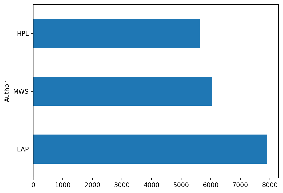
We can observe that the excerpts from the 3 authors are not necessarily balanced within the dataset. If this corpus is later used for modeling, it will be important to account for this imbalance.

(
  horror
  .value_counts('Author')
  .plot(kind = "barh")
)

3 Initial Frequency Analysis

The standard approach in statistics—starting with descriptive analysis before modeling—also applies to text data analysis. Text mining therefore begins with a statistical analysis to determine the structure of the corpus.

Before diving into a systematic analysis of each author’s lexical field, we will first focus on a single word: fear.

3.1 Targeted Exploration

Tip

The exercise below presents a graphical representation called a waffle chart. This is a better alternative to pie charts, which are misleading because the human eye can be easily deceived by their shape, which does not accurately represent proportions.

Exercise 1: Word Frequency

First, we will focus on our Anglo-Saxon corpus (horror)

1. Count the number of sentences, for each author, in which the word fear appears.
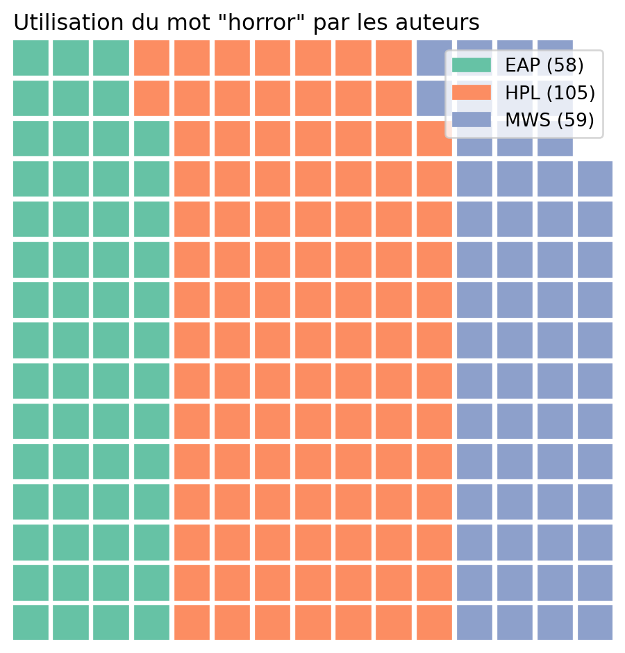
2. Use pywaffle to generate the charts below that visually summarize the number of occurrences of the word “fear” by author.
3. Repeat the analysis with the word “horror”.

The resulting count should be as follows

	wordtoplot
Author
EAP	70
HPL	160
MWS	211

This produces the following waffle chart:

Figure 3.1: Répartition du terme fear dans le corpus de nos trois auteurs

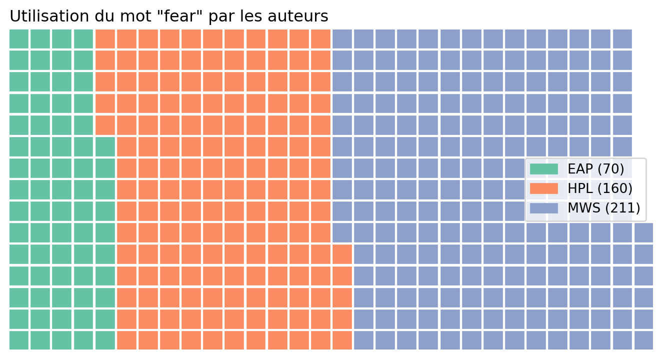
This clearly highlights the imbalance in our dataset when focusing on the term “fear”, with Mary Shelley accounting for nearly 50% of the observations.

If we repeat the analysis with the term “horror”, we get the following figure:

Figure 3.2: Répartition du terme horror dans le corpus de nos trois auteurs

3.2 Converting Text into Tokens

In the previous exercise, we performed a one-off search, which doesn’t scale well. To generalize this approach, a corpus is typically broken down into independent semantic units: tokens.

Tip

We will need to import several ready-to-use corpora to work with the NLTK or SpaCy libraries. The instructions below will help you retrieve all these resources.

To retrieve all our ready-to-use NLTK corpora, we do the following

import nltk
nltk.download('stopwords')
nltk.download('punkt')
nltk.download('punkt_tab')
nltk.download('genesis')
nltk.download('wordnet')
nltk.download('omw-1.4')

For SpaCy, it is necessary to use the following command line:

!python -m spacy download fr_core_news_sm
!python -m spacy download en_core_web_sm

Rather than implementing an inefficient tokenizer yourself, it is more appropriate to use one from a specialized library. Historically, the simplest choice was to use the tokenizer from NLTK, the classic Python text mining library:

from nltk.tokenize import word_tokenize
word_tokenize(dumas[10000:10500])

As we can see, this library lacks detail and has some inconsistencies: j'y étais is split into 4 tokens (['j', "'", 'y', 'étais']) whereas l'acheter remains a single token. NLTK is an English-centric library, and its tokenization algorithm is not always well-suited to French grammar rules. In such cases, it is better to use SpaCy, the more modern library for this kind of task. Besides being well-documented, it is better adapted to non-English languages. As shown in the documentation example on tokenizers, its algorithm provides a certain level of sophistication:

Example of a tokenization algorithm

It can be applied in the following way:

import spacy
from spacy.tokenizer import Tokenizer
nlp = spacy.load("fr_core_news_sm")
doc = nlp(dumas[10000:10500])

text_tokenized = []
for token in doc:
    text_tokenized += [token.text]

", ".join(text_tokenized)

" , mes, yeux, ., --vous, avez, donc, vu, l', empereur, aussi, ?, --il, est, entré, chez, le, maréchal, pendant, que, j', y, étais, ., --et, vous, lui, avez, parlé, ?, --c', est, -, à, -, dire, que, c', est, lui, qui, m', a, parlé, ,, monsieur, ,, dit, dantès, en, souriant, ., --et, que, vous, a, -t, -il, dit, ?, --il, m', a, fait, des, questions, sur, le, bâtiment, ,, sur, l', époque, de, son, départ, pour, marseille, ,, sur, la, route, qu', il, avait, suivie, et, sur, la, cargaison, qu', il, portait, ., je, crois, que, s', il, eût, été, vide, ,, et, que, j', en, eusse, été, le, maître, ,, son, intention, eût, été, de, l', acheter, ;, mais, je, lu"

As we can see, there are still many elements cluttering our corpus structure, starting with punctuation. However, we will be able to easily remove these later on, as we will see.

3.3 Word Cloud: A First Generalized Analysis

At this point, we still have no clear sense of the structure of our corpus: word count, most frequent words, etc.

To get an idea of the corpus structure, we can start by counting word distribution in Dumas’ work. Let’s begin with the first 30,000 words and count the unique words:

from collections import Counter

doc = nlp(dumas[:30000])

# Extract tokens, convert to lowercase and filter out punctuation and spaces
tokens = [token.text.lower() for token in doc if not token.is_punct and not token.is_space]

# Count the frequency of each token
token_counts = Counter(tokens)

There are already many different words in the beginning of the work.

len(token_counts)

1401

We can observe the high dimensionality of the corpus, with nearly 1,500 unique words in the first 30,000 words of Dumas’ work.

token_count_all = list(token_counts.items())

# Create a DataFrame from the list of tuples
token_count_all = pd.DataFrame(token_count_all, columns=['word', 'count'])

If we look at the distribution of word frequencies—an analysis we will extend later when discussing Zipf’s law—we can see that many words are unique (nearly half), that the frequency density drops off quickly, and that we should focus more on the tail of the distribution than the following figure allows:

from plotnine import *
(
  ggplot(token_count_all) +
  geom_histogram(aes(x = "count")) +
  scale_x_log10()
)

/opt/conda/lib/python3.12/site-packages/plotnine/stats/stat_bin.py:109: PlotnineWarning: 'stat_bin()' using 'bins = 42'. Pick better value with 'binwidth'.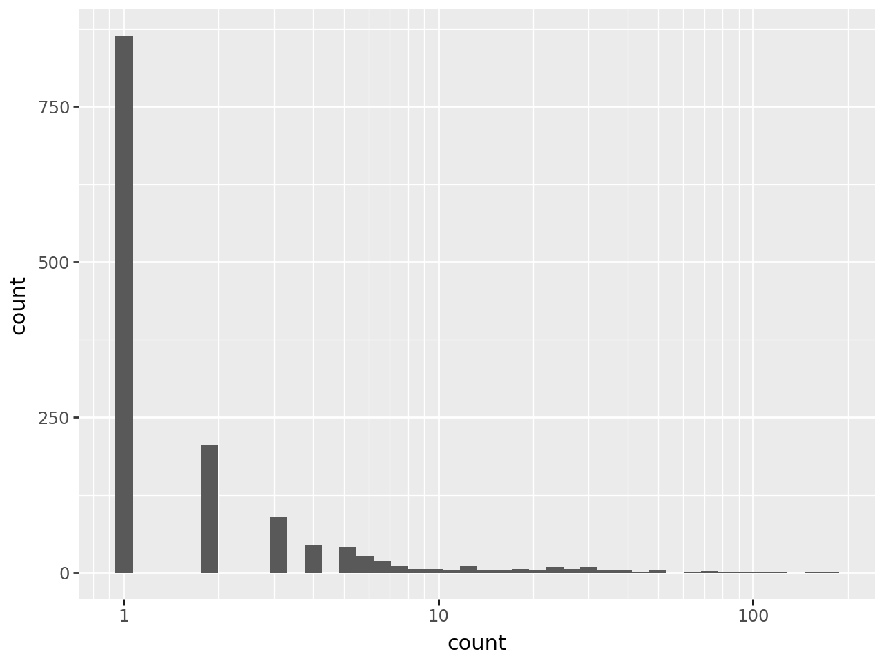

Now, if we look at the 25 most frequent words, we can see that they are not very informative for analyzing the meaning of our document:

# Sort the tokens by frequency in descending order
sorted_token_counts = token_counts.most_common(25)
sorted_token_counts = pd.DataFrame(sorted_token_counts, columns=['word', 'count'])

/tmp/ipykernel_7061/3224890599.py:18: MapWithoutReturnDtypeWarning: Calling `map_elements` without specifying `return_dtype` can lead to unpredictable results. Specify `return_dtype` to silence this warning.
/tmp/ipykernel_7061/3224890599.py:23: MapWithoutReturnDtypeWarning: Calling `map_elements` without specifying `return_dtype` can lead to unpredictable results. Specify `return_dtype` to silence this warning.

Mot	Nombre d'occurrences
de	176
le	149
et	124
à	116
l'	102
que	100
vous	88
la	83
il	81
un	77
je	73
en	70
est	61
qui	53
dantès	53
d'	50
dit	50
les	49
du	46
a	41
ne	37
n'	37
mon	37
son	36
pas	36
Nombre d'apparitions sur les 30 000 premiers caractères du Comte de Monte Cristo

If we represent this ranking graphically

(
    ggplot(sorted_token_counts, aes(x='word', y='count')) +
    geom_point(stat='identity', size = 3, color = "red") +
    scale_x_discrete(
      limits=sorted_token_counts.sort_values("count")["word"].tolist()
    ) +
    coord_flip() +
    theme_minimal() +
    labs(title='Word Frequency', x='Word', y='Count')
)

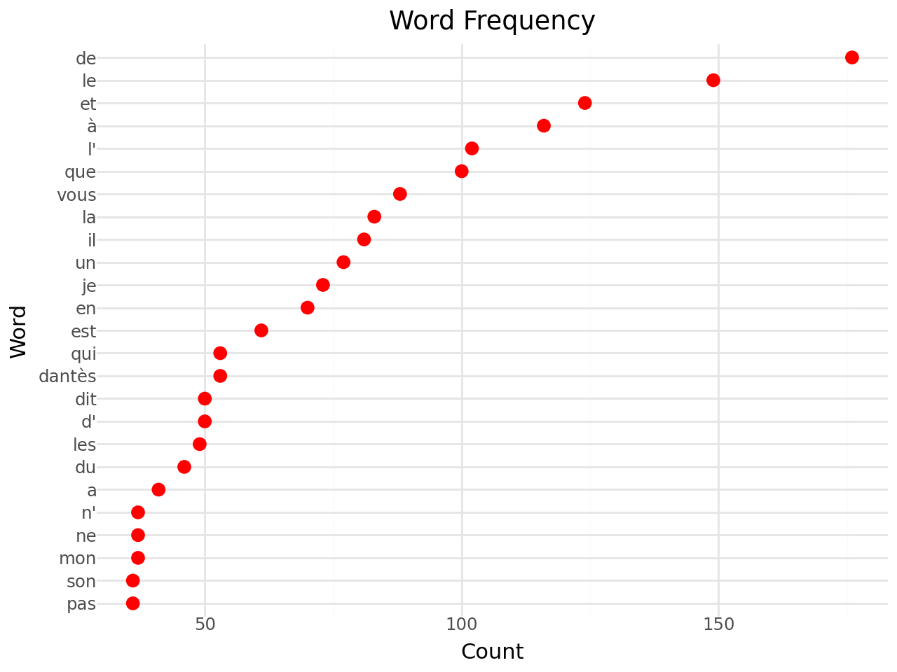
We will focus on these filler words later on, as it will be important to account for them in our deeper document analyses.

Through these word counts, we’ve gained a first intuition about the nature of our corpus. However, a more visual approach would be helpful to gain further insight. Word clouds are convenient graphical representations for visualizing the most frequent words—when used appropriately. Word clouds are very easy to implement in Python with the Wordcloud module. Some formatting parameters even allow the shape of the cloud to be adjusted to match an image.

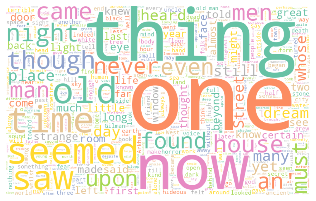
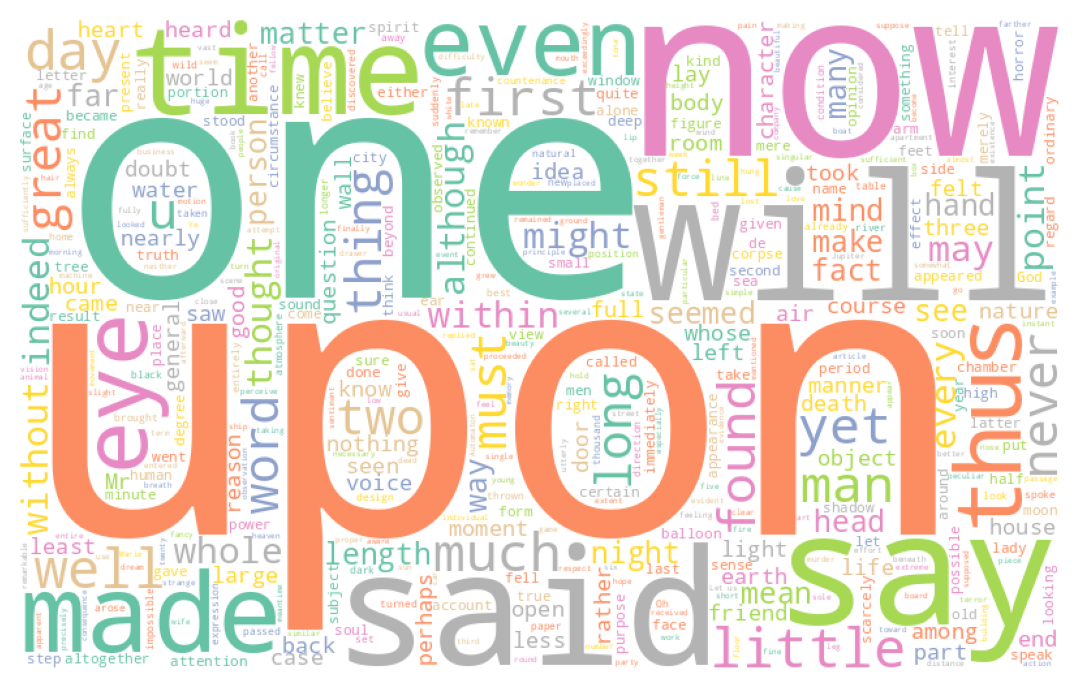
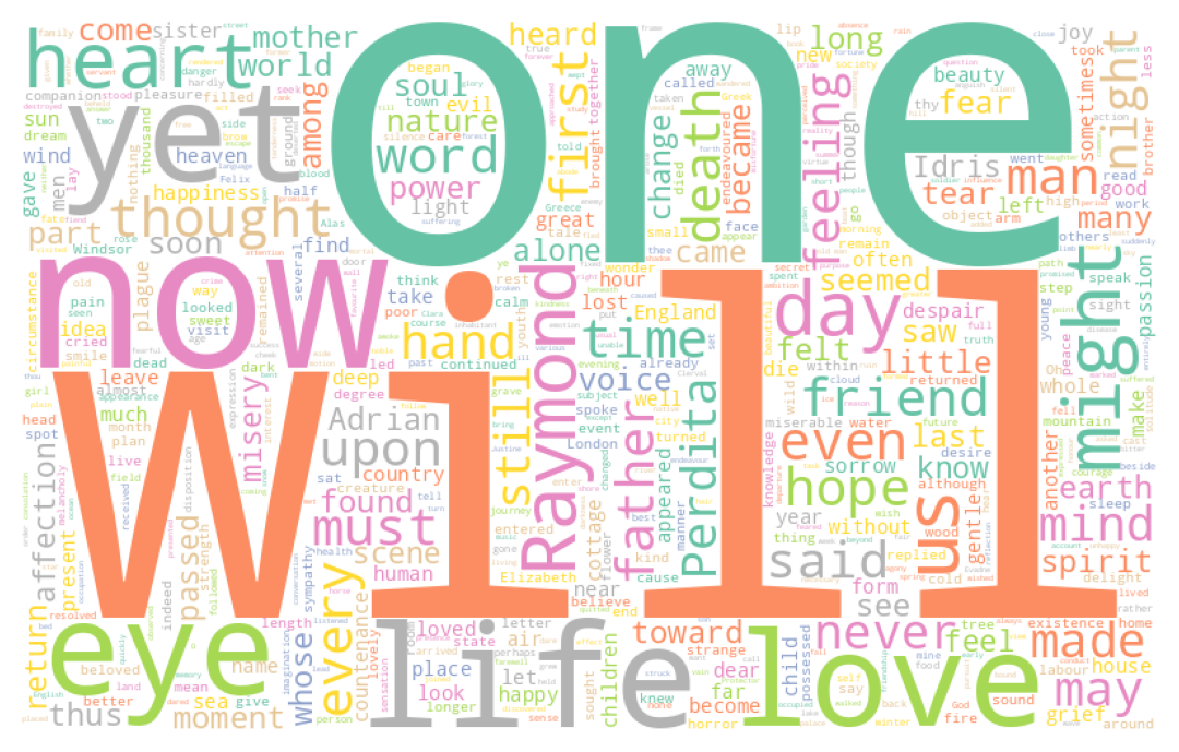
Exercise 2: Wordcloud

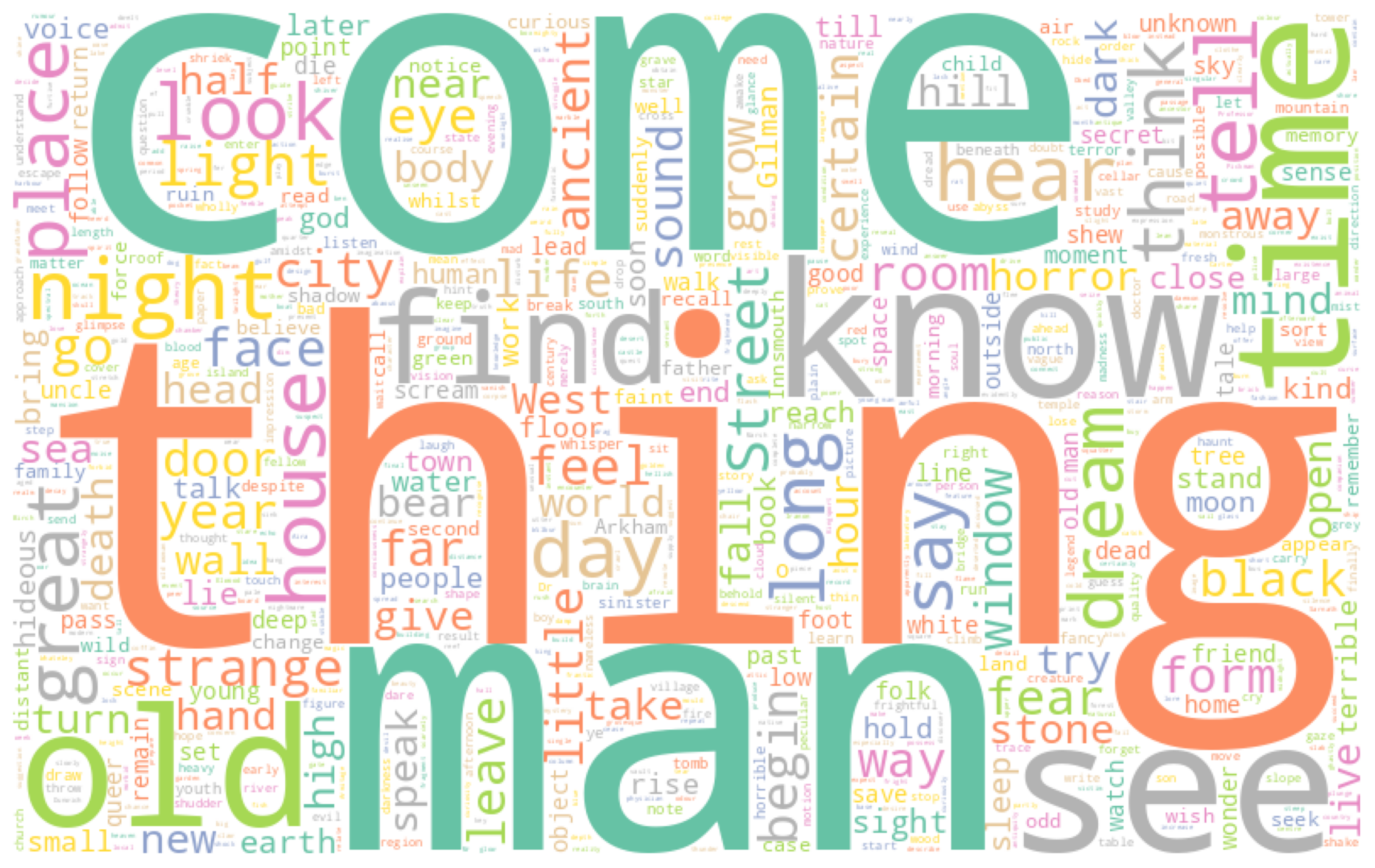
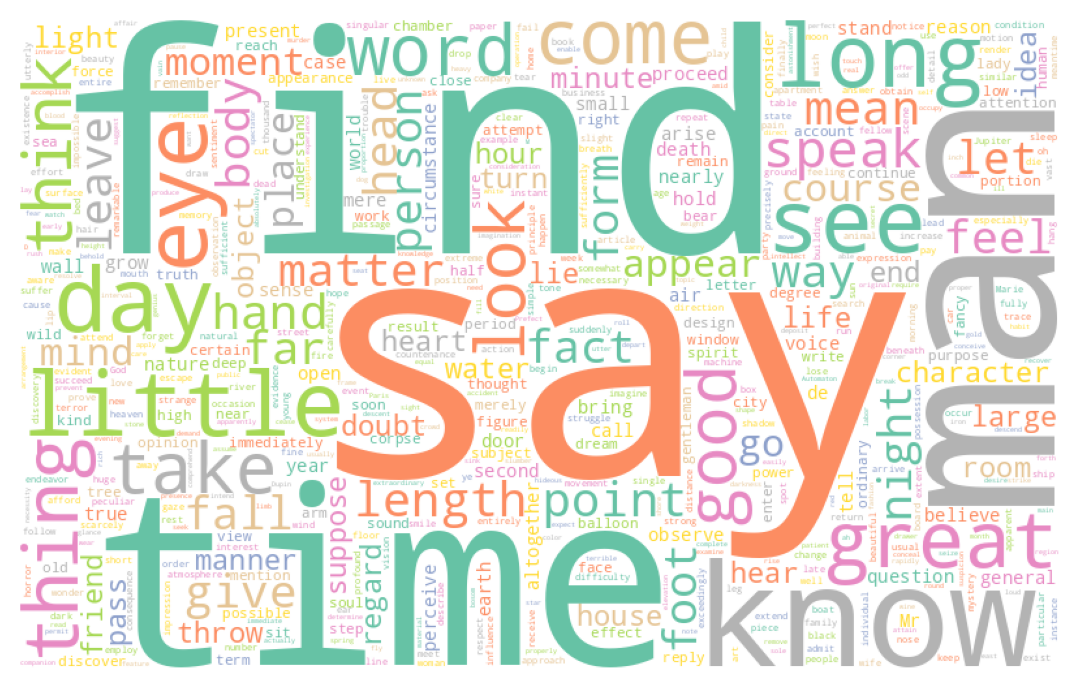
1. Using the wordCloud function, create three word clouds to represent the most commonly used words by each author in the horror corpus¹.
2. Create a word cloud for the dumas corpus using a mask like the one below.

Example mask for question 2

Image URL: https://minio.lab.sspcloud.fr/lgaliana/generative-art/pythonds/book.png

The word clouds generated for question 1 are as follows:

Figure 3.3: Lovercraft

Figure 3.4: Poe

Figure 3.5: Shelley

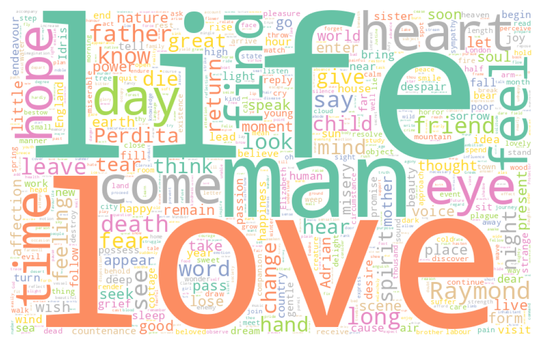
Whereas the one generated from Dumas’ work takes the shape

Figure 3.6: Nuage de mot produit à partir du Comte de Monte Cristo

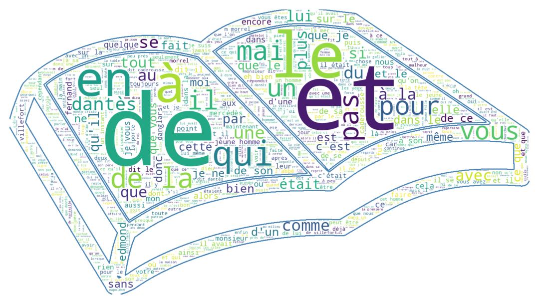
If it wasn’t already obvious, these visualizations clearly show the need to clean our text. For instance, in the case of Dumas’ work, the name of the main character, Dantès, is obscured by various articles or connecting words that interfere with the analysis. In the Anglo-Saxon corpus, similar terms like “the”, “of”, etc., dominate.

These words are called stop words. This is a clear example of why text should be cleaned before analysis (unless one is interested in Zipf’s law, see the next exercise).

3.4 Aside: Zipf’s Law

In the 1930s, Zipf observed a statistical regularity in Joyce’s Ulysses. The most frequent word appeared \(x\) times, the second most frequent word appeared half as often, the third a third as often, and so on. Statistically, this means that the frequency of occurrence \(f(n_i)\) of a word is related to its rank \(n_i\) in the frequency order by a law of the form:

\[f(n_i) = c/n_i\]

where \(c\) is a constant.

More generally, Zipf’s law can be derived from an exponentially decreasing frequency distribution: \(f(n_i) = cn_{i}^{-k}\). Empirically, this means that we can use Poisson regressions to estimate the law’s parameters, following the specification:

\[ \mathbb{E}\bigg( f(n_i)|n_i \bigg) = \exp(\beta_0 + \beta_1 \log(n_i)) \]

Generalized linear models (GLMs) allow us to perform this type of regression. In Python, they are available via the statsmodels package, whose outputs are heavily inspired by specialized econometric software such as Stata.

count_words = pd.DataFrame({'counter' : horror
    .groupby('Author')
    .apply(lambda s: ' '.join(s['Text']).split())
    .apply(lambda s: Counter(s))
    .apply(lambda s: s.most_common())
    .explode()}
)
count_words[['word','count']] = pd.DataFrame(count_words['counter'].tolist(), index=count_words.index)
count_words = count_words.reset_index()

count_words = count_words.assign(
    tot_mots_auteur = lambda x: (x.groupby("Author")['count'].transform('sum')),
    freq = lambda x: x['count'] /  x['tot_mots_auteur'],
    rank = lambda x: x.groupby("Author")['count'].transform('rank', ascending = False)
)

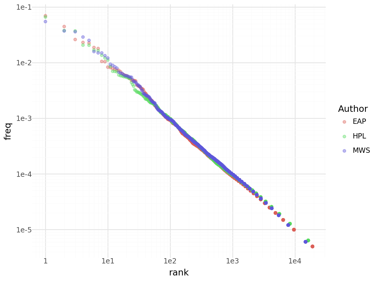
/tmp/ipykernel_7061/4009929367.py:3: DeprecationWarning: DataFrameGroupBy.apply operated on the grouping columns. This behavior is deprecated, and in a future version of pandas the grouping columns will be excluded from the operation. Either pass `include_groups=False` to exclude the groupings or explicitly select the grouping columns after groupby to silence this warning.

Let’s begin by visualizing the relationship between frequency and rank:

from plotnine import *

g = (
    ggplot(count_words) +
    geom_point(aes(y = "freq", x = "rank", color = 'Author'), alpha = 0.4) +
    scale_x_log10() + scale_y_log10() +
    theme_minimal()
)

We do indeed observe a log-linear relationship between the two in the plot:

Using statsmodels, let’s formally verify this relationship:

import statsmodels.api as sm
import numpy as np

exog = sm.add_constant(np.log(count_words['rank'].astype(float)))

model = sm.GLM(count_words['freq'].astype(float), exog, family = sm.families.Poisson()).fit()

# Afficher les résultats du modèle
print(model.summary())

                 Generalized Linear Model Regression Results                  
==============================================================================
Dep. Variable:                   freq   No. Observations:                69301
Model:                            GLM   Df Residuals:                    69299
Model Family:                 Poisson   Df Model:                            1
Link Function:                    Log   Scale:                          1.0000
Method:                          IRLS   Log-Likelihood:                -23.011
Date:                Mon, 26 May 2025   Deviance:                     0.065676
Time:                        18:57:55   Pearson chi2:                   0.0656
No. Iterations:                     5   Pseudo R-squ. (CS):          0.0002431
Covariance Type:            nonrobust                                         
==============================================================================
                 coef    std err          z      P>|z|      [0.025      0.975]
------------------------------------------------------------------------------
const         -2.4388      1.089     -2.239      0.025      -4.574      -0.303
rank          -0.9831      0.189     -5.196      0.000      -1.354      -0.612
==============================================================================

The regression coefficient is close to 1, which suggests a nearly log-linear relationship between rank and word frequency. In other words, the most used word occurs twice as often as the second most frequent word, which occurs three times more than the third, and so on. This law is indeed empirically observed in this corpus of three authors.

4 Text Cleaning

4.1 Removing Stop Words

As we have seen, whether in French or English, a number of connecting words, while grammatically necessary, carry little informational value and prevent us from identifying the main information-bearing words in our corpus.

Therefore, it is necessary to clean our corpus by removing such terms. This cleaning process goes beyond simply removing words; it’s also an opportunity to eliminate other problematic tokens, such as punctuation.

Let’s start by downloading the stopwords corpus

import nltk
nltk.download('stopwords')

[nltk_data] Downloading package stopwords to /github/home/nltk_data...
[nltk_data]   Package stopwords is already up-to-date!

True

The list of English stopwords in NLTK is as follows:

from nltk.corpus import stopwords
", ".join(stopwords.words("english"))

"a, about, above, after, again, against, ain, all, am, an, and, any, are, aren, aren't, as, at, be, because, been, before, being, below, between, both, but, by, can, couldn, couldn't, d, did, didn, didn't, do, does, doesn, doesn't, doing, don, don't, down, during, each, few, for, from, further, had, hadn, hadn't, has, hasn, hasn't, have, haven, haven't, having, he, he'd, he'll, her, here, hers, herself, he's, him, himself, his, how, i, i'd, if, i'll, i'm, in, into, is, isn, isn't, it, it'd, it'll, it's, its, itself, i've, just, ll, m, ma, me, mightn, mightn't, more, most, mustn, mustn't, my, myself, needn, needn't, no, nor, not, now, o, of, off, on, once, only, or, other, our, ours, ourselves, out, over, own, re, s, same, shan, shan't, she, she'd, she'll, she's, should, shouldn, shouldn't, should've, so, some, such, t, than, that, that'll, the, their, theirs, them, themselves, then, there, these, they, they'd, they'll, they're, they've, this, those, through, to, too, under, until, up, ve, very, was, wasn, wasn't, we, we'd, we'll, we're, were, weren, weren't, we've, what, when, where, which, while, who, whom, why, will, with, won, won't, wouldn, wouldn't, y, you, you'd, you'll, your, you're, yours, yourself, yourselves, you've"

The list provided by SpaCy is more comprehensive (we have already downloaded the en_core_web_sm corpus in question):

nlp_english = spacy.load('en_core_web_sm')
stop_words_english = nlp_english.Defaults.stop_words
", ".join(stop_words_english)

"always, ever, off, seems, was, sometimes, beyond, more, ‘re, he, whereby, elsewhere, above, part, behind, them, no, hence, whether, somehow, latterly, say, 've, well, something, whereas, yours, beside, becomes, afterwards, out, give, between, whither, amount, front, unless, due, seem, how, himself, two, about, being, for, also, 'd, down, see, will, namely, whence, the, quite, must, her, my, ten, who, us, by, put, its, ’re, three, per, else, within, twelve, did, below, most, few, get, not, never, same, several, some, full, neither, do, from, hundred, thereby, they, sometime, then, ’s, ’m, made, it, serious, have, your, alone, because, nor, seemed, until, our, throughout, side, as, if, this, already, during, make, hereupon, itself, once, what, hers, seeming, yourselves, four, myself, formerly, next, that, though, were, thru, move, whoever, take, which, where, only, into, eleven, too, please, up, wherever, last, over, along, amongst, a, towards, before, noone, ‘m, anywhere, can, former, whom, than, are, you, ourselves, these, with, still, be, all, yet, another, has, on, upon, when, am, name, and, his, through, fifty, indeed, ca, own, whole, doing, besides, further, whenever, herself, twenty, among, third, such, ‘ve, enough, eight, become, ’ve, whereupon, ‘ll, others, there, to, ours, thus, forty, nobody, five, rather, themselves, under, after, whereafter, could, nowhere, therefore, least, becoming, fifteen, mine, i, bottom, but, even, moreover, either, except, anything, used, became, much, thence, using, n‘t, just, since, meanwhile, yourself, re, both, around, without, very, across, often, in, thereupon, first, however, those, ‘d, or, regarding, show, call, of, nevertheless, been, their, n't, beforehand, one, ’ll, anyway, other, herein, empty, hereafter, top, should, everywhere, nothing, many, me, does, ’d, whatever, everything, toward, against, while, sixty, whose, onto, now, 'll, everyone, anyone, anyhow, cannot, had, perhaps, 's, 're, n’t, almost, although, keep, go, him, at, somewhere, none, six, each, may, 'm, really, would, nine, here, why, any, various, via, otherwise, is, back, every, again, she, wherein, ‘s, less, might, hereby, therein, latter, someone, we, so, done, an, together, mostly, thereafter"

This time, if we look at the list of French stopwords in NLTK:

", ".join(stopwords.words("french"))

'au, aux, avec, ce, ces, dans, de, des, du, elle, en, et, eux, il, ils, je, la, le, les, leur, lui, ma, mais, me, même, mes, moi, mon, ne, nos, notre, nous, on, ou, par, pas, pour, qu, que, qui, sa, se, ses, son, sur, ta, te, tes, toi, ton, tu, un, une, vos, votre, vous, c, d, j, l, à, m, n, s, t, y, été, étée, étées, étés, étant, étante, étants, étantes, suis, es, est, sommes, êtes, sont, serai, seras, sera, serons, serez, seront, serais, serait, serions, seriez, seraient, étais, était, étions, étiez, étaient, fus, fut, fûmes, fûtes, furent, sois, soit, soyons, soyez, soient, fusse, fusses, fût, fussions, fussiez, fussent, ayant, ayante, ayantes, ayants, eu, eue, eues, eus, ai, as, avons, avez, ont, aurai, auras, aura, aurons, aurez, auront, aurais, aurait, aurions, auriez, auraient, avais, avait, avions, aviez, avaient, eut, eûmes, eûtes, eurent, aie, aies, ait, ayons, ayez, aient, eusse, eusses, eût, eussions, eussiez, eussent'

We can see that this list is not very extensive and could benefit from being more complete. The one from SpaCy is more in line with what we would expect.

stop_words_french = nlp.Defaults.stop_words
", ".join(stop_words_french)

"quatorze, son, environ, à, delà, certaine, un, auxquelles, du, sur, permet, en, dix-neuf, sans, lequel, quant-à-soi, quarante, y, pourrait, soit, etant, qui, maintenant, ô, desquelles, nous-mêmes, lui-même, egalement, hou, cinquante, vos, voici, elles-memes, pourrais, t', semblent, hé, sont, suivants, leur, celle-ci, quatre-vingt, les, eu, vers, hem, ont, suivre, semblable, merci, cinq, parfois, differentes, anterieures, aurait, devers, tel, sauf, quelques, sent, vingt, peux, pres, ma, unes, avait, notre, quant, si, pour, différents, toutes, da, assez, lès, avec, ou, et, quelqu'un, sera, mille, peu, troisièmement, bas, ces, dont, voilà, facon, hormis, suit, reste, également, plutot, il, plutôt, parmi, desquels, m’, auraient, allaient, chacun, souvent, nombreux, puisque, ça, moi-meme, font, restent, hui, ni, seize, elle-même, mêmes, auront, suffisante, ce, sienne, cent, étant, seuls, aussi, quoi, seules, stop, leurs, alors, treize, different, huitième, quels, quelque, telles, ho, est, hi, precisement, sien, préalable, specifique, eux-mêmes, abord, enfin, autrui, meme, vous, dire, tente, celles, nombreuses, soi-même, pas, mien, dedans, serait, quiconque, car, celui-ci, diverses, antérieur, anterieure, parlent, te, proche, nôtres, différent, as, neuvième, onze, d’, suivantes, mais, puis, étaient, laquelle, nôtre, relativement, chaque, était, depuis, dix-huit, toute, quand, soi-meme, différente, suivant, basee, ouias, ouste, sa, feront, huit, spécifique, comment, directement, quel, neanmoins, uns, pouvait, malgré, attendu, deuxième, derrière, na, tiennes, encore, sept, aura, dixième, tend, a, dits, doivent, autres, lorsque, apres, aux, desormais, toi-même, nous, ci, hue, la, lui, durant, vé, ouverts, lui-meme, dessous, celles-là, té, suis, faisant, auxquels, étais, dix, revoilà, ès, jusqu, c’, suivante, bat, celle-là, donc, tenant, avant, suffit, seul, elle-meme, avons, on, deja, etait, hors, ne, cependant, plusieurs, ton, quinze, doit, gens, que, onzième, longtemps, l', toi, douzième, sixième, ta, allons, votres, differente, certaines, tres, parler, celui, soixante, des, retour, elle, nouveau, miens, comme, duquel, sinon, deux, désormais, mienne, moindres, antérieures, après, etre, afin, troisième, etais, eux, trente, lesquelles, l’, seule, devra, où, cela, miennes, ait, ai, rendre, m', soi, peuvent, jusque, t’, telle, toi-meme, relative, auquel, juste, ils, ouvert, deuxièmement, très, celui-là, ceci, rend, première, procedant, personne, possible, premier, exactement, précisement, envers, tes, je, suffisant, effet, seulement, ainsi, semble, possibles, quatrièmement, j', i, seraient, vas, celle, celles-la, etc, tellement, ses, celle-la, tien, directe, s', differents, cette, parle, quatre, siennes, celles-ci, eh, tenir, elles, etaient, avais, nos, vont, cinquantaine, hep, dehors, maint, surtout, pense, dix-sept, ayant, tout, houp, divers, avoir, or, quelles, avaient, fais, moi-même, o, malgre, selon, devant, revoici, tels, prealable, certes, entre, notamment, vôtre, semblaient, près, siens, être, vôtres, cinquantième, revoila, chez, parce, va, cet, premièrement, debout, c', me, tu, même, outre, quelle, autre, derriere, moins, lesquels, es, aupres, par, ah, diverse, compris, toujours, partant, qu’, qu', douze, chacune, certains, touchant, quatrième, quoique, concernant, dans, se, dessus, pourquoi, ceux-ci, dit, voila, mon, trois, cinquième, d', faisaient, ceux, plus, nul, memes, anterieur, sous, autrement, ha, une, ceux-là, vu, importe, excepté, votre, specifiques, déjà, pendant, tienne, au, j’, elles-mêmes, quelconque, septième, dite, six, le, peut, lors, vais, aie, vous-mêmes, seront, dès, mes, pu, restant, fait, certain, là, façon, sait, via, tiens, celui-la, combien, laisser, déja, â, ouverte, tant, moi, tous, n’, spécifiques, dejà, s’, de, néanmoins, n', différentes, antérieure"

Exercise 3: Text Cleaning

1. Take Dumas’ work and clean it using Spacy. Generate the word cloud again and draw your conclusions.
2. Perform the same task on the Anglo-Saxon dataset. Ideally, you should be able to use the SpaCy pipeline functionality.

# Function to clean the text
def clean_text(doc):
    # Tokenize, remove stop words and punctuation, and lemmatize
    cleaned_tokens = [
        token.lemma_ for token in doc if not token.is_stop and not token.is_punct
    ]
    # Join tokens back into a single string
    cleaned_text = " ".join(cleaned_tokens)
    return cleaned_text

Ces retraitements commencent à porter leurs fruits puisque des mots ayant plus de sens commencent à se dégager, notamment les noms des personnages (Dantès, Danglart, etc.):

Figure 4.1: Nuage de mot produit à partir du Comte de Monte Cristo après nettoyage

Figure 4.2: Lovercraft

Figure 4.3: Poe

Figure 4.4: Shelley

4.2 Stemming and Lemmatization

To go further in text harmonization, it is possible to establish equivalence classes between words. For example, when conducting frequency analysis, one might want to treat “cheval” and “chevaux” as equivalent. Depending on the context, different forms of the same word (plural, singular, conjugated) can be treated as equivalent and replaced with a canonical form.

There are two main approaches:

• Lemmatization, which requires knowledge of grammatical roles (example: “chevaux” becomes “cheval”);
• Stemming, which is more rudimentary but faster, especially when dealing with spelling errors. In this case, “chevaux” might become “chev”, but that could also match “chevet” or “cheveux”.

This approach has the advantage of reducing the vocabulary size that both the computer and modeler must handle. Several stemming algorithms exist, including the Porter Stemming Algorithm and the Snowball Stemming Algorithm.

Note

To access the necessary corpus for lemmatization, you need to download it the first time using the following commands:

import nltk
nltk.download('wordnet')
nltk.download('omw-1.4')

Let’s take this character string:

"naples. comme d'habitude, un pilote côtier partit aussitôt du port, rasa le château d'if, et alla aborder le navire entre le cap de morgion et l'île de rion. aussitôt, co"

The stemmed version is as follows:

"napl,.,comm,d'habitud,,,un,pilot,côti,part,aussitôt,du,port,,,ras,le,château,d'if,,,et,alla,abord,le,navir,entre,le,cap,de,morgion,et,l'îl,de,rion,.,aussitôt,,,co"

At this stage, the words become less intelligible for humans but can still be understandable for machines. This choice is not trivial, and its relevance depends on the specific use case.

Lemmatizers allow for more nuanced harmonization. They rely on knowledge bases, such as WordNet, an open lexical database. For instance, the words “women”, “daughters”, and “leaves” will be lemmatized as follows:

from nltk.stem import WordNetLemmatizer
lemm = WordNetLemmatizer()

for word in ["women","daughters", "leaves"]:
    print(f"The lemmatized form of {word} is: {lemm.lemmatize(word)}")

The lemmatized form of women is: woman
The lemmatized form of daughters is: daughter
The lemmatized form of leaves is: leaf

Exercise 4: Lemmatization with nltk

Following the previous example, use a WordNetLemmatizer on the dumas[1030:1200] corpus and observe the result.

The lemmatized version of this small excerpt from Dumas’ work is as follows:

"naples, ., comme, d'habitude, ,, un, pilote, côtier, partit, aussitôt, du, port, ,, rasa, le, château, d'if, ,, et, alla, aborder, le, navire, entre, le, cap, de, morgion, et, l'île, de, rion, ., aussitôt, ,, co"

4.3 Limitation

In frequency-based approaches, where the goal is to find similarity between texts based on term co-occurrence, the question of forming equivalence classes is fundamental. Words are either identical or different—there is no subtle gradation. For instance, one must decide whether “python” and “pythons” are equivalent or not, without any nuance distinguishing “pythons”, “anaconda”, or “table” from “python”. Modern approaches, which no longer rely solely on word frequency, allow for more nuance in synthesizing the information present in textual data.

Informations additionnelles

environment files have been tested on.

Latest built version: 2025-05-26

Python version used:

'3.12.6 | packaged by conda-forge | (main, Sep 30 2024, 18:08:52) [GCC 13.3.0]'

Package	Version
affine	2.4.0
aiobotocore	2.15.1
aiohappyeyeballs	2.4.3
aiohttp	3.10.8
aioitertools	0.12.0
aiosignal	1.3.1
alembic	1.13.3
altair	5.4.1
aniso8601	9.0.1
annotated-types	0.7.0
anyio	4.9.0
appdirs	1.4.4
archspec	0.2.3
asttokens	2.4.1
attrs	24.2.0
babel	2.17.0
bcrypt	4.2.0
beautifulsoup4	4.12.3
black	24.8.0
blinker	1.8.2
blis	1.3.0
bokeh	3.5.2
boltons	24.0.0
boto3	1.35.23
botocore	1.35.23
branca	0.7.2
Brotli	1.1.0
bs4	0.0.2
cachetools	5.5.0
cartiflette	0.1.9
Cartopy	0.24.1
catalogue	2.0.10
cattrs	24.1.3
certifi	2025.4.26
cffi	1.17.1
charset-normalizer	3.3.2
chromedriver-autoinstaller	0.6.4
click	8.1.7
click-plugins	1.1.1
cligj	0.7.2
cloudpathlib	0.21.1
cloudpickle	3.0.0
colorama	0.4.6
comm	0.2.2
commonmark	0.9.1
conda	24.9.1
conda-libmamba-solver	24.7.0
conda-package-handling	2.3.0
conda_package_streaming	0.10.0
confection	0.1.5
contextily	1.6.2
contourpy	1.3.0
cryptography	43.0.1
cycler	0.12.1
cymem	2.0.11
cytoolz	1.0.0
dask	2024.9.1
dask-expr	1.1.15
databricks-sdk	0.33.0
dataclasses-json	0.6.7
debugpy	1.8.6
decorator	5.1.1
Deprecated	1.2.14
diskcache	5.6.3
distributed	2024.9.1
distro	1.9.0
docker	7.1.0
duckdb	1.1.1
en_core_web_sm	3.8.0
entrypoints	0.4
et_xmlfile	2.0.0
exceptiongroup	1.2.2
executing	2.1.0
fastexcel	0.14.0
fastjsonschema	2.21.1
fiona	1.10.1
Flask	3.0.3
folium	0.19.6
fontawesomefree	6.6.0
fonttools	4.54.1
fr_core_news_sm	3.8.0
frozendict	2.4.4
frozenlist	1.4.1
fsspec	2024.9.0
geographiclib	2.0
geopandas	1.0.1
geoplot	0.5.1
geopy	2.4.1
gitdb	4.0.11
GitPython	3.1.43
google-auth	2.35.0
graphene	3.3
graphql-core	3.2.4
graphql-relay	3.2.0
graphviz	0.20.3
great-tables	0.12.0
greenlet	3.1.1
gunicorn	22.0.0
h11	0.16.0
h2	4.1.0
hpack	4.0.0
htmltools	0.6.0
httpcore	1.0.9
httpx	0.28.1
httpx-sse	0.4.0
hyperframe	6.0.1
idna	3.10
imageio	2.37.0
importlib_metadata	8.5.0
importlib_resources	6.4.5
inflate64	1.0.1
ipykernel	6.29.5
ipython	8.28.0
itsdangerous	2.2.0
jedi	0.19.1
Jinja2	3.1.4
jmespath	1.0.1
joblib	1.4.2
jsonpatch	1.33
jsonpointer	3.0.0
jsonschema	4.23.0
jsonschema-specifications	2025.4.1
jupyter-cache	1.0.0
jupyter_client	8.6.3
jupyter_core	5.7.2
kaleido	0.2.1
kiwisolver	1.4.7
langchain	0.3.25
langchain-community	0.3.9
langchain-core	0.3.61
langchain-text-splitters	0.3.8
langcodes	3.5.0
langsmith	0.1.147
language_data	1.3.0
lazy_loader	0.4
libmambapy	1.5.9
locket	1.0.0
loguru	0.7.3
lxml	5.4.0
lz4	4.3.3
Mako	1.3.5
mamba	1.5.9
mapclassify	2.8.1
marisa-trie	1.2.1
Markdown	3.6
markdown-it-py	3.0.0
MarkupSafe	2.1.5
marshmallow	3.26.1
matplotlib	3.9.2
matplotlib-inline	0.1.7
mdurl	0.1.2
menuinst	2.1.2
mercantile	1.2.1
mizani	0.11.4
mlflow	2.16.2
mlflow-skinny	2.16.2
msgpack	1.1.0
multidict	6.1.0
multivolumefile	0.2.3
munkres	1.1.4
murmurhash	1.0.13
mypy_extensions	1.1.0
narwhals	1.41.0
nbclient	0.10.0
nbformat	5.10.4
nest_asyncio	1.6.0
networkx	3.3
nltk	3.9.1
numpy	2.1.2
opencv-python-headless	4.10.0.84
openpyxl	3.1.5
opentelemetry-api	1.16.0
opentelemetry-sdk	1.16.0
opentelemetry-semantic-conventions	0.37b0
orjson	3.10.18
outcome	1.3.0.post0
OWSLib	0.33.0
packaging	24.1
pandas	2.2.3
paramiko	3.5.0
parso	0.8.4
partd	1.4.2
pathspec	0.12.1
patsy	0.5.6
Pebble	5.1.1
pexpect	4.9.0
pickleshare	0.7.5
pillow	10.4.0
pip	24.2
platformdirs	4.3.6
plotly	5.24.1
plotnine	0.13.6
pluggy	1.5.0
polars	1.8.2
preshed	3.0.10
prometheus_client	0.21.0
prometheus_flask_exporter	0.23.1
prompt_toolkit	3.0.48
protobuf	4.25.3
psutil	6.0.0
ptyprocess	0.7.0
pure_eval	0.2.3
py7zr	0.22.0
pyarrow	17.0.0
pyarrow-hotfix	0.6
pyasn1	0.6.1
pyasn1_modules	0.4.1
pybcj	1.0.6
pycosat	0.6.6
pycparser	2.22
pycryptodomex	3.23.0
pydantic	2.11.5
pydantic_core	2.33.2
pydantic-settings	2.9.1
Pygments	2.18.0
PyNaCl	1.5.0
pynsee	0.1.8
pyogrio	0.10.0
pyOpenSSL	24.2.1
pyparsing	3.1.4
pyppmd	1.1.1
pyproj	3.7.0
pyshp	2.3.1
PySocks	1.7.1
python-dateutil	2.9.0
python-dotenv	1.0.1
python-magic	0.4.27
pytz	2024.1
pyu2f	0.1.5
pywaffle	1.1.1
PyYAML	6.0.2
pyzmq	26.2.0
pyzstd	0.16.2
querystring_parser	1.2.4
rasterio	1.4.3
referencing	0.36.2
regex	2024.9.11
requests	2.32.3
requests-cache	1.2.1
requests-toolbelt	1.0.0
retrying	1.3.4
rich	14.0.0
rpds-py	0.25.1
rsa	4.9
rtree	1.4.0
ruamel.yaml	0.18.6
ruamel.yaml.clib	0.2.8
s3fs	2024.9.0
s3transfer	0.10.2
scikit-image	0.24.0
scikit-learn	1.5.2
scipy	1.13.0
seaborn	0.13.2
selenium	4.33.0
setuptools	74.1.2
shapely	2.0.6
shellingham	1.5.4
six	1.16.0
smart-open	7.1.0
smmap	5.0.0
sniffio	1.3.1
sortedcontainers	2.4.0
soupsieve	2.5
spacy	3.8.4
spacy-legacy	3.0.12
spacy-loggers	1.0.5
SQLAlchemy	2.0.35
sqlparse	0.5.1
srsly	2.5.1
stack-data	0.6.2
statsmodels	0.14.4
tabulate	0.9.0
tblib	3.0.0
tenacity	9.0.0
texttable	1.7.0
thinc	8.3.6
threadpoolctl	3.5.0
tifffile	2025.5.24
toolz	1.0.0
topojson	1.9
tornado	6.4.1
tqdm	4.67.1
traitlets	5.14.3
trio	0.30.0
trio-websocket	0.12.2
truststore	0.9.2
typer	0.16.0
typing_extensions	4.13.2
typing-inspect	0.9.0
typing-inspection	0.4.1
tzdata	2024.2
Unidecode	1.4.0
url-normalize	2.2.1
urllib3	2.4.0
uv	0.7.8
wasabi	1.1.3
wcwidth	0.2.13
weasel	0.4.1
webdriver-manager	4.0.2
websocket-client	1.8.0
Werkzeug	3.0.4
wheel	0.44.0
wordcloud	1.9.3
wrapt	1.16.0
wsproto	1.2.0
xgboost	2.1.1
xlrd	2.0.1
xyzservices	2024.9.0
yarl	1.13.1
yellowbrick	1.5
zict	3.0.0
zipp	3.20.2
zstandard	0.23.0

View file history

md`Ce fichier a été modifié __${table_commit.length}__ fois depuis sa création le ${creation_string} (dernière modification le ${last_modification_string})`

creation = d3.min(
  table_commit.map(d => new Date(d.Date))
)

last_modification = d3.max(
  table_commit.map(d => new Date(d.Date))
)

creation_string = creation.toLocaleString("fr", {
  "day": "numeric",
  "month": "long",
  "year": "numeric"
})

last_modification_string = last_modification.toLocaleString("fr", {
  "day": "numeric",
  "month": "long",
  "year": "numeric"
})

html`<div>${git_history_table}</div>`

html`<div>${git_history_plot}</div>`

SHA	Date	Author	Description
df498c79	2025-05-24 19:10:07	Lino Galiana	uv friendly pipeline (#605)
d6b67125	2025-05-23 18:03:48	Lino Galiana	Traduction des chapitres NLP (#603)
4181dab1	2024-12-06 13:16:36	lgaliana	Transition
1b7188a1	2024-12-05 13:21:11	lgaliana	Embedding chapter
c641de05	2024-08-22 11:37:13	Lino Galiana	A series of fix for notebooks that were bugging (#545)
0908656f	2024-08-20 16:30:39	Lino Galiana	English sidebar (#542)
5108922f	2024-08-08 18:43:37	Lino Galiana	Improve notebook generation and tests on PR (#536)
8d23a533	2024-07-10 18:45:54	Julien PRAMIL	Modifs 02_exoclean.qmd (#523)
75950080	2024-07-08 17:24:29	Julien PRAMIL	Changes into NLP/01_intro.qmd (#517)
56b6442d	2024-07-08 15:05:57	Lino Galiana	Version anglaise du chapitre numpy (#516)
a3dc832c	2024-06-24 16:15:19	Lino Galiana	Improve homepage images (#508)
e660d769	2024-06-19 14:31:09	linogaliana	improve output NLP 1
4f41cf6a	2024-06-14 15:00:41	Lino Galiana	Une partie sur les sacs de mots plus cohérente (#501)
06d003a1	2024-04-23 10:09:22	Lino Galiana	Continue la restructuration des sous-parties (#492)
005d89b8	2023-12-20 17:23:04	Lino Galiana	Finalise l’affichage des statistiques Git (#478)
3437373a	2023-12-16 20:11:06	Lino Galiana	Améliore l’exercice sur le LASSO (#473)
4cd44f35	2023-12-11 17:37:50	Antoine Palazzolo	Relecture NLP (#474)
deaafb6f	2023-12-11 13:44:34	Thomas Faria	Relecture Thomas partie NLP (#472)
4c060a17	2023-12-01 17:44:17	Lino Galiana	Update book image location
1f23de28	2023-12-01 17:25:36	Lino Galiana	Stockage des images sur S3 (#466)
a1ab3d94	2023-11-24 10:57:02	Lino Galiana	Reprise des chapitres NLP (#459)
a7711832	2023-10-09 11:27:45	Antoine Palazzolo	Relecture TD2 par Antoine (#418)
154f09e4	2023-09-26 14:59:11	Antoine Palazzolo	Des typos corrigées par Antoine (#411)
80823022	2023-08-25 17:48:36	Lino Galiana	Mise à jour des scripts de construction des notebooks (#395)
3bdf3b06	2023-08-25 11:23:02	Lino Galiana	Simplification de la structure 🤓 (#393)
f2905a7d	2023-08-11 17:24:57	Lino Galiana	Introduction de la partie NLP (#388)
78ea2cbd	2023-07-20 20:27:31	Lino Galiana	Change titles levels (#381)
a9b384ed	2023-07-18 18:07:16	Lino Galiana	Sépare les notebooks (#373)
29ff3f58	2023-07-07 14:17:53	linogaliana	description everywhere
f21a24d3	2023-07-02 10:58:15	Lino Galiana	Pipeline Quarto & Pages 🚀 (#365)
164fa689	2022-11-30 09:13:45	Lino Galiana	Travail partie NLP (#328)
f10815b5	2022-08-25 16:00:03	Lino Galiana	Notebooks should now look more beautiful (#260)
494a85ae	2022-08-05 14:49:56	Lino Galiana	Images featured ✨ (#252)
d201e3cd	2022-08-03 15:50:34	Lino Galiana	Pimp la homepage ✨ (#249)
12965bac	2022-05-25 15:53:27	Lino Galiana	:launch: Bascule vers quarto (#226)
9c71d6e7	2022-03-08 10:34:26	Lino Galiana	Plus d’éléments sur S3 (#218)
3299f1d9	2022-01-08 16:50:11	Lino Galiana	Clean NLP notebooks (#215)
495599d7	2021-12-19 18:33:05	Lino Galiana	Des éléments supplémentaires dans la partie NLP (#202)
4f675284	2021-12-12 08:37:21	Lino Galiana	Improve website appareance (#194)
2a8809fb	2021-10-27 12:05:34	Lino Galiana	Simplification des hooks pour gagner en flexibilité et clarté (#166)
04f8b8f6	2021-09-08 11:55:35	Lino Galiana	echo = FALSE sur la page tuto NLP
048e3dd6	2021-09-02 18:36:23	Lino Galiana	Fix problem with Dumas corpus (#134)
2e4d5862	2021-09-02 12:03:39	Lino Galiana	Simplify badges generation (#130)
49e2826f	2021-05-13 18:11:20	Lino Galiana	Corrige quelques images n’apparaissant pas (#108)
4cdb759c	2021-05-12 10:37:23	Lino Galiana	:sparkles: :star2: Nouveau thème hugo :snake: :fire: (#105)
48ed9d25	2021-05-01 08:58:58	Lino Galiana	lien mort corrigé
7f9f97bc	2021-04-30 21:44:04	Lino Galiana	🐳 + 🐍 New workflow (docker 🐳) and new dataset for modelization (2020 🇺🇸 elections) (#99)
d164635d	2020-12-08 16:22:00	Lino Galiana	:books: Première partie NLP (#87)

git_history_table = Inputs.table(
  table_commit,
  {
    format: {
      SHA: x => md`[${x}](${github_repo}/commit/${x})`,
      Description: x => md`${replacePullRequestPattern(x, github_repo)}`,
      /*Date: x => x.toLocaleString("fr", {
        "month": "numeric",
        "day": "numeric",
        "year": "numeric"
        })
      */
    }
  }
)

git_history_plot = Plot.plot({
  marks: [
    Plot.ruleY([0], {stroke: "royalblue"}),
    Plot.dot(
          table_commit,
          Plot.pointerX({x: (d) => new Date(d.date), y: 0, stroke: "red"})),
    Plot.dot(table_commit, {x: (d) => new Date(d.Date), y: 0, fill: "royalblue"})
  ]
})

function replacePullRequestPattern(inputString, githubRepo) {
    // Use a regular expression to match the pattern #digit
    var pattern = /#(\d+)/g;

    // Replace the pattern with ${github_repo}/pull/#digit
    var replacedString = inputString.replace(pattern, '[#$1](' + githubRepo + '/pull/$1)');

    return replacedString;
}

github_repo = "https://github.com/linogaliana/python-datascientist"

table_commit = {

// Get the HTML table by its class name
var table = document.querySelector('.commit-table');

// Check if the table exists
if (table) {
    // Initialize an array to store the table data
    var dataArray = [];

    // Extract headers from the first row
    var headers = [];
    for (var i = 0; i < table.rows[0].cells.length; i++) {
        headers.push(table.rows[0].cells[i].textContent.trim());
    }

    // Iterate through the rows, starting from the second row
    for (var i = 1; i < table.rows.length; i++) {
        var row = table.rows[i];
        var rowData = {};

        // Iterate through the cells in the row
        for (var j = 0; j < row.cells.length; j++) {
            // Use headers as keys and cell content as values
            rowData[headers[j]] = row.cells[j].textContent.trim();
        }

        // Push the rowData object to the dataArray
        dataArray.push(rowData);
    }
  }

  return dataArray

}

// Get the element with class 'git-details'
{
  var gitDetails = document.querySelector('.commit-table');

  // Check if the element exists
  if (gitDetails) {
      // Hide the element
      gitDetails.style.display = 'none';
  }
}

Plot = require('@observablehq/plot@0.6.12/dist/plot.umd.min.js')

Footnotes

1. To obtain the same results as shown below, you can set the argument random_state=21.