!pip install geopandas openpyxl plotnine plotlyIf you want to try the examples in this tutorial:

The previous chapter aimed to propose a first model to understand the counties where the Republican Party wins. The variable of interest was bimodal (win or lose), placing us within the framework of a classification model.
Now, using the same data, we will propose a regression model to explain the Republican Party’s score. The variable is thus continuous. We will ignore the fact that its bounds lie between 0 and 100, meaning that to be rigorous, we would need to transform the scale so that the data fits within this interval.
Machine learning materials in this course uses a unique dataset, presented in the introduction. All examples are based on US county level presidential election results combined with sociodemographic variables. Source code for data ingestion is available on Github.
import requests

url = 'https://raw.githubusercontent.com/linogaliana/python-datascientist/main/content/modelisation/get_data.py'
r = requests.get(url, allow_redirects=True)
open('getdata.py', 'wb').write(r.content)

import getdata
votes = getdata.create_votes_dataframes()
This chapter will use several modeling packages, the main ones being Scikit and Statsmodels.
Here is a suggested import for all these packages.
import numpy as np
from sklearn.linear_model import LinearRegression
from sklearn.model_selection import train_test_split
import sklearn.metrics
import matplotlib.pyplot as plt
import seaborn as sns
import pandas as pd
1 General Principle
The general principle of regression consists of finding a law \(h_\theta(X)\) such that
\[ h_\theta(X) = \mathbb{E}_\theta(Y|X) \]
This formalization is extremely general and is not limited to linear regression.
In econometrics, regression offers an alternative to maximum likelihood methods and moment methods. Regression encompasses a very broad range of methods, depending on the family of models (parametric, non-parametric, etc.) and model structures.
1.1 Linear Regression
This is the simplest way to represent the law \(h_\theta(X)\) as a linear combination of variables \(X\) and parameters \(\theta\). In this case,
\[ \mathbb{E}_\theta(Y|X) = X\beta \]
This relationship is, under this formulation, theoretical. It must be estimated from the observed data \(y\). The method of least squares aims to minimize the quadratic error between the prediction and the observed data (which explains why regression can be seen as a Machine Learning problem). In general, the method of least squares seeks to find the set of parameters \(\theta\) such that
\[ \theta = \arg \min_{\theta \in \Theta} \mathbb{E}\bigg[ \left( y - h_\theta(X) \right)^2 \bigg] \]
Which, in the context of linear regression, is expressed as follows:
\[ \beta = \arg\min \mathbb{E}\bigg[ \left( y - X\beta \right)^2 \bigg] \]
When the theoretical model (\(\mathbb{E}_\theta(Y|X) = X\beta\)) is applied to data, the model is formalized as follows:
\[ Y = X\beta + \epsilon \]
With a certain distribution of the noise \(\epsilon\) that depends on the assumptions made. For example, with \(\epsilon \sim \mathcal{N}(0,\sigma^2)\) i.i.d., the estimator \(\beta\) obtained is equivalent to the Maximum Likelihood Estimator, whose asymptotic theory ensures unbiasedness and minimum variance (Cramer-Rao bound).
1.1.1 Application
Under the guidance of the heirs of Siegfried (1913), our objective in this chapter is to explain and predict the Republican score based on some socioeconomic variables. Unlike the previous chapter, where we focused on a binary outcome (Republican victory/defeat), this time we will model the Republican score directly.
The next exercise aims to demonstrate how to perform linear regression using scikit.
In this area, statsmodels is significantly more comprehensive, as the following exercise will demonstrate.
The main advantage of performing regressions with scikit is the ability to compare the results of linear regression with other regression models in the context of selecting the best predictive model.
TipExercise 1a: Linear Regression with scikit
- Using a few variables, for example, ‘Unemployment_rate_2019’, ‘Median_Household_Income_2021’, ‘Percent of adults with less than a high school diploma, 2018-22’, “Percent of adults with a bachelor’s degree or higher, 2018-22”, explain the variable
per_gopusing a training sampleX_trainprepared beforehand.
⚠️ Use the variable Median_Household_Income_2021 in log form; otherwise, its scale might dominate and obscure other effects.
Display the values of the coefficients, including the constant.
Evaluate the relevance of the model using \(R^2\) and assess the fit quality with the MSE.
Plot a scatter plot of observed values and prediction errors. Do you observe any specification issues?
In question 4, it can be observed that the distribution of errors is clearly not random with respect to \(X\).
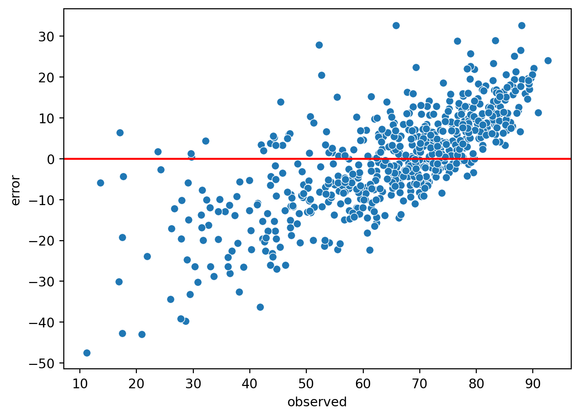
The model therefore suffers from a specification issue, so work will need to be done on the selected variables later. Before that, we can redo this exercise using the statsmodels package.
TipExercise 1b: Linear Regression with statsmodels
This exercise aims to demonstrate how to perform linear regression using statsmodels, which offers features more similar to those of R and less oriented toward Machine Learning.
The goal is still to explain the Republican score based on a few variables.
Using a few variables, for example, ‘Unemployment_rate_2019’, ‘Median_Household_Income_2021’, ‘Percent of adults with less than a high school diploma, 2015-19’, “Percent of adults with a bachelor’s degree or higher, 2015-19”, explain the variable
per_gop.
⚠️ Use the variableMedian_Household_Income_2021inlogform; otherwise, its scale might dominate and obscure other effects.Display a regression table.
Evaluate the model’s relevance using the R^2.
Use the
formulaAPI to regress the Republican score as a function of the variableUnemployment_rate_2019,Unemployment_rate_2019squared, and the log ofMedian_Household_Income_2021.
R2: 0.43016652968844415
TipTip
To generate a well-formatted table for a report in \(\LaTeX\), you can use the method Summary.as_latex. For an HTML report, you can use Summary.as_html.
NoteNote
Users of R will find many familiar features in statsmodels, particularly the ability to use a formula to define a regression. The philosophy of statsmodels is similar to that which influenced the construction of R’s stats and MASS packages: providing a general-purpose library with a wide range of models.
However, statsmodels benefits from being more modern compared to R’s packages. Since the 1990s, R packages aiming to provide missing features in stats and MASS have proliferated, while statsmodels, born in the 2010s, only had to propose a general framework (the generalized estimating equations) to encompass these models.
1.2 La régression logistique
We applied our linear regression to a continuous outcome variable.
How do we handle a binary distribution?
In this case, \(\mathbb{E}_{\theta} (Y|X) = \mathbb{P}_{\theta} (Y = 1|X)\).
Logistic regression can be seen as a linear probability model:
\[ \text{logit}\bigg(\mathbb{E}_{\theta}(Y|X)\bigg) = \text{logit}\bigg(\mathbb{P}_{\theta}(Y = 1|X)\bigg) = X\beta \]
The \(\text{logit}\) function is \(]0,1[ \to \mathbb{R}: p \mapsto \log(\frac{p}{1-p})\).
It allows a probability to be transformed into \(\mathbb{R}\). Its reciprocal function is the sigmoid (\(\frac{1}{1 + e^{-x}}\)), a central concept in Deep Learning.
It should be noted that probabilities are not observed; what is observed is the binary outcome (0/1). This leads to two different perspectives on logistic regression:
- In econometrics, interest lies in the latent model that determines the choice of the outcome. For example, if observing the choice to participate in the labor market, the goal is to model the factors determining this choice;
- In Machine Learning, the latent model is only necessary to classify observations into the correct category.
Parameter estimation for \(\beta\) can be performed using maximum likelihood or regression, both of which are equivalent under certain assumptions.
TipExercise 2a: Logistic Regression with scikit
Using scikit with training and test samples:
- Evaluate the effect of the already-used variables on the probability of Republicans winning. Display the values of the coefficients.
- Derive a confusion matrix and a measure of model quality.
- Remove regularization using the
penaltyparameter. What effect does this have on the estimated parameters?
TipExercise 2b: Logistic Regression with statsmodels
Using training and test samples:
- Evaluate the effect of the already-used variables on the probability of Republicans winning.
- Perform a likelihood ratio test regarding the inclusion of the (log)-income variable.
The p-value of the likelihood ratio test being close to 1 means that the log-income variable almost certainly adds information to the model.
TipTip
The test statistic is: \[ LR = -2\log\bigg(\frac{\mathcal{L}_{\theta}}{\mathcal{L}_{\theta_0}}\bigg) = -2(\mathcal{l}_{\theta} - \mathcal{l}_{\theta_0}) \]
2 Going Further
This chapter only introduces the concepts of regression in a very introductory way. To expand on this, it is recommended to explore further based on your interests and needs.
In the field of machine learning, the main areas for deeper exploration are:
- Alternative regression models like random forests.
- Boosting and bagging methods to learn how multiple models can be trained jointly and their predictions combined democratically to converge on better decisions than a single model.
- Issues related to model explainability, a very active research area, to better understand the decision criteria of models.
In the field of econometrics, the main areas for deeper exploration are:
- Generalized linear models to explore regression with more general assumptions than those we have made so far;
- Hypothesis testing to delve deeper into these questions beyond our likelihood ratio test.
References
Informations additionnelles
NotePython environment
This site was built automatically through a Github action using the Quarto
The environment used to obtain the results is reproducible via uv. The pyproject.toml file used to build this environment is available on the linogaliana/python-datascientist repository
pyproject.toml
[project]
name = "python-datascientist"
version = "0.1.0"
description = "Source code for Lino Galiana's Python for data science course"
readme = "README.md"
requires-python = ">=3.13,<3.14"
dependencies = [
    "altair>=6.0.0",
    "cartiflette",
    "contextily==1.6.2",
    "duckdb>=0.10.1",
    "folium>=0.19.6",
    "gdal==3.11.4",
    "graphviz==0.20.3",
    "great-tables>=0.12.0",
    "gt-extras>=0.0.8",
    "ipykernel>=6.29.5",
    "jupyter>=1.1.1",
    "jupyter-cache>=1.0.0",
    "kaleido>=0.2.1",
    "langchain-community>=0.3.27",
    "loguru==0.7.3",
    "markdown>=3.8",
    "nbclient>=0.10.0",
    "nbformat>=5.10.4",
    "nltk>=3.9.1",
    "pandas>=3.0",
    "pip>=25.1.1",
    "plotly>=6.1.2",
    "plotnine>=0.15",
    "polars>=1.8.2",
    "pyarrow>=17.0.0",
    "pynsee>=0.1.8",
    "python-dotenv>=1.0.1",
    "python-frontmatter>=1.1.0",
    "pywaffle>=1.1.1",
    "requests>=2.32.3",
    "scikit-image>=0.24.0",
    "scikit-learn>=1.8.0",
    "scipy>=1.13.0",
    "seaborn>=0.13.2",
    "selenium<4.39.0",
    "spacy>=3.8.4",
    "webdriver-manager>=4.0.2",
    "wordcloud==1.9.3",
]

[tool.uv.sources]
cartiflette = { git = "https://github.com/inseefrlab/cartiflette" }
gdal = [
  { index = "gdal-wheels", marker = "sys_platform == 'linux'" },
  { index = "geospatial_wheels", marker = "sys_platform == 'win32'" },
]

[[tool.uv.index]]
name = "geospatial_wheels"
url = "https://nathanjmcdougall.github.io/geospatial-wheels-index/"
explicit = true

[[tool.uv.index]]
name = "gdal-wheels"
url = "https://gitlab.com/api/v4/projects/61637378/packages/pypi/simple"
explicit = true

[dependency-groups]
dev = [
    "nb-clean>=4.0.1",
]
To use exactly the same environment (version of Python and packages), please refer to the documentation for uv.
NoteFile history
| SHA | Date | Author | Description |
|---|---|---|---|
| d56f6e9e | 2025-11-25 08:30:59 | lgaliana | Un petit coup de neuf sur les consignes et corrections pandas related |
| 94648290 | 2025-07-22 18:57:48 | Lino Galiana | Fix boxes now that it is better supported by jupyter (#628) |
| 91431fa2 | 2025-06-09 17:08:00 | Lino Galiana | Improve homepage hero banner (#612) |
| 48dccf14 | 2025-01-14 21:45:34 | lgaliana | Fix bug in modeling section |
| d4f89590 | 2024-12-20 14:36:20 | lgaliana | format fstring R2 |
| 8c8ca4c0 | 2024-12-20 10:45:00 | lgaliana | Traduction du chapitre clustering |
| a5ecaedc | 2024-12-20 09:36:42 | Lino Galiana | Traduction du chapitre modélisation (#582) |
| ff0820bc | 2024-11-27 15:10:39 | lgaliana | Mise en forme chapitre régression |
| 06d003a1 | 2024-04-23 10:09:22 | Lino Galiana | Continue la restructuration des sous-parties (#492) |
| 8c316d0a | 2024-04-05 19:00:59 | Lino Galiana | Fix cartiflette deprecated snippets (#487) |
| 005d89b8 | 2023-12-20 17:23:04 | Lino Galiana | Finalise l’affichage des statistiques Git (#478) |
| 7d12af8b | 2023-12-05 10:30:08 | linogaliana | Modularise la partie import pour l’avoir partout |
| 417fb669 | 2023-12-04 18:49:21 | Lino Galiana | Corrections partie ML (#468) |
| a06a2689 | 2023-11-23 18:23:28 | Antoine Palazzolo | 2ème relectures chapitres ML (#457) |
| 889a71ba | 2023-11-10 11:40:51 | Antoine Palazzolo | Modification TP 3 (#443) |
| 154f09e4 | 2023-09-26 14:59:11 | Antoine Palazzolo | Des typos corrigées par Antoine (#411) |
| 9a4e2267 | 2023-08-28 17:11:52 | Lino Galiana | Action to check URL still exist (#399) |
| a8f90c2f | 2023-08-28 09:26:12 | Lino Galiana | Update featured paths (#396) |
| 3bdf3b06 | 2023-08-25 11:23:02 | Lino Galiana | Simplification de la structure 🤓 (#393) |
| 78ea2cbd | 2023-07-20 20:27:31 | Lino Galiana | Change titles levels (#381) |
| 29ff3f58 | 2023-07-07 14:17:53 | linogaliana | description everywhere |
| f21a24d3 | 2023-07-02 10:58:15 | Lino Galiana | Pipeline Quarto & Pages 🚀 (#365) |
| 58c71287 | 2023-06-11 21:32:03 | Lino Galiana | change na subset (#362) |
| 2ed4aa78 | 2022-11-07 15:57:31 | Lino Galiana | Reprise 2e partie ML + Règle problème mathjax (#319) |
| f10815b5 | 2022-08-25 16:00:03 | Lino Galiana | Notebooks should now look more beautiful (#260) |
| 494a85ae | 2022-08-05 14:49:56 | Lino Galiana | Images featured ✨ (#252) |
| d201e3cd | 2022-08-03 15:50:34 | Lino Galiana | Pimp la homepage ✨ (#249) |
| 12965bac | 2022-05-25 15:53:27 | Lino Galiana | :launch: Bascule vers quarto (#226) |
| 9c71d6e7 | 2022-03-08 10:34:26 | Lino Galiana | Plus d’éléments sur S3 (#218) |
| c3bf4d42 | 2021-12-06 19:43:26 | Lino Galiana | Finalise debug partie ML (#190) |
| fb14d406 | 2021-12-06 17:00:52 | Lino Galiana | Modifie l’import du script (#187) |
| 37ecfa3c | 2021-12-06 14:48:05 | Lino Galiana | Essaye nom différent (#186) |
| 5d0a5e38 | 2021-12-04 07:41:43 | Lino Galiana | MAJ URL script recup data (#184) |
| 5c104904 | 2021-12-03 17:44:08 | Lino Galiana | Relec (antuki?) partie modelisation (#183) |
| 2a8809fb | 2021-10-27 12:05:34 | Lino Galiana | Simplification des hooks pour gagner en flexibilité et clarté (#166) |
| 2e4d5862 | 2021-09-02 12:03:39 | Lino Galiana | Simplify badges generation (#130) |
| 4cdb759c | 2021-05-12 10:37:23 | Lino Galiana | :sparkles: :star2: Nouveau thème hugo :snake: :fire: (#105) |
| 7f9f97bc | 2021-04-30 21:44:04 | Lino Galiana | 🐳 + 🐍 New workflow (docker 🐳) and new dataset for modelization (2020 🇺🇸 elections) (#99) |
| 59eadf58 | 2020-11-12 16:41:46 | Lino Galiana | Correction des typos partie ML (#81) |
| 347f50f3 | 2020-11-12 15:08:18 | Lino Galiana | Suite de la partie machine learning (#78) |
| 671f75a4 | 2020-10-21 15:15:24 | Lino Galiana | Introduction au Machine Learning (#72) |
References
Siegfried, André. 1913. Tableau Politique de La France de l’ouest Sous La Troisième république: 102 Cartes Et Croquis, 1 Carte Hors Texte. A. Colin.
Citation
BibTeX citation:
@book{galiana2025,
  author = {Galiana, Lino},
  title = {Python Pour La Data Science},
  date = {2025},
  url = {https://pythonds.linogaliana.fr/},
  doi = {10.5281/zenodo.8229676},
  langid = {en}
}
For attribution, please cite this work as:
Galiana, Lino. 2025. Python Pour La Data Science. https://doi.org/10.5281/zenodo.8229676.