!pip install spacy
!python -m spacy download en_core_web_sm
!python -m spacy download fr_core_news_smIf you want to try the examples in this tutorial:

To move forward in this chapter, we need to perform some preliminary installations:
It is also useful to define the following function, taken from our previous chapter:
def clean_text(doc):
    # Tokenize, remove stop words and punctuation, and lemmatize
    cleaned_tokens = [token.lemma_ for token in doc if not token.is_stop and not token.is_punct]
    # Join tokens back into a single string
    cleaned_text = ' '.join(cleaned_tokens)
    return cleaned_text
1 Introduction
Previously, we saw the importance of cleaning data to filter down the volume of information present in unstructured data. The goal of this chapter is to deepen our understanding of the frequency-based approach applied to text data. We will explore how this frequentist analysis helps summarize the information contained within a text corpus. We’ll also look at how to refine the bag of words approach by taking into account the order or proximity of terms within a sentence.
1.1 Data
We will reuse the Anglo-Saxon dataset from the previous chapter, which includes texts from gothic authors Edgar Allan Poe (EAP), HP Lovecraft (HPL), and Mary Wollstonecraft Shelley (MWS).
import pandas as pd

url='https://github.com/GU4243-ADS/spring2018-project1-ginnyqg/raw/master/data/spooky.csv'
#1. Import des données
horror = pd.read_csv(url,encoding='latin-1')
#2. Majuscules aux noms des colonnes
horror.columns = horror.columns.str.capitalize()
#3. Retirer le prefixe id
horror['ID'] = horror['Id'].str.replace("id","")
horror = horror.set_index('Id')
2 The TF-IDF Measure (term frequency - inverse document frequency)
2.1 The Document-Term Matrix
As mentioned earlier, we construct a synthetic representation of our corpus as a bag of words, where words are sampled more or less frequently depending on their appearance frequency. This is, of course, a simplified representation of reality: word sequences are not just random independent words.
However, before addressing those limitations, we should complete the bag-of-words approach. The most characteristic representation of this paradigm is the document-term matrix, mainly used to compare corpora. It involves creating a matrix where each document is represented by the presence or absence of terms in our corpus. The idea is to count how often words (terms, in columns) appear in each sentence or phrase (documents, in rows). This matrix then becomes a numerical representation of the text data.
Consider a corpus made up of the following three sentences:
- The practice of knitting and crocheting
- Passing on the passion for stamps
- Living off one’s passion”
The corresponding document-term matrix is:
| Sentence | and | crocheting | for | knitting | living | of | one’s | on | passion | passing | practice | stamps | the |
|---|---|---|---|---|---|---|---|---|---|---|---|---|---|
| The practice of knitting and crocheting | 1 | 1 | 0 | 1 | 0 | 1 | 0 | 0 | 0 | 0 | 1 | 0 | 1 |
| Passing on the passion for stamps | 0 | 0 | 1 | 0 | 0 | 0 | 0 | 1 | 1 | 1 | 0 | 1 | 1 |
| Living off one’s passion | 0 | 0 | 0 | 0 | 1 | 0 | 1 | 0 | 1 | 0 | 0 | 0 | 0 |
Each sentence in the corpus is associated with a numeric vector. For instance,
the sentence “La pratique du tricot et du crochet”, which is meaningless to a machine on its own, becomes a numeric vector it can interpret: [1, 0, 2, 1, 1, 0, 1, 0, 0, 0, 1, 0]. This numeric vector is a sparse representation of language, since each document (row) will only contain a small portion of the total vocabulary (all columns). Words that do not appear in a document are represented as zeros, hence a sparse vector. As we’ll see later, this numeric representation is very different from modern embedding approaches, which are based on dense representations.
2.2 Use for Information Retrieval
Different documents can then be compared based on these measures. This is one of the methods used by search engines, although the most advanced ones rely on far more sophisticated approaches. The tf-idf metric (term frequency–inverse document frequency) allows for calculating a relevance score between a search term and a document using two components:
\[ \text{tf-idf}(t, d, D) = \text{tf}(t, d) \times \text{idf}(t, D) \]
Let \(t\) be a specific term (e.g., a word), \(d\) a specific document, and \(D\) the entire set of documents in the corpus.
The
tfcomponent computes a function that increases with the frequency of the search term in the document under consideration;The
idfcomponent computes a function that decreases with the frequency of the term across the entire document set (or corpus).The first part (term frequency, TF) is the frequency of occurrence of term \(t\) in document \(d\). There are normalization strategies available to avoid biasing the score in favor of longer documents.
\[ \text{tf}(t, d) = \frac{f_{t,d}}{\sum_{t' \in d} f_{t',d}} \]
where \(f_{t,d}\) is the raw count of how many times term \(t\) appears in document \(d\), and the denominator is the total number of terms in document \(d\).
- The second part (inverse document frequency, IDF) measures the rarity—or conversely, the commonness—of a term across the corpus. If \(N\) is the total number of documents in the corpus \(D\), this part of the metric is given by
\[ \text{idf}(t, D) = \log \left( \frac{N}{|\{d \in D : t \in d\}|} \right) \]
The denominator \(( |\{d \in D : t \in d\}| )\) corresponds to the number of documents in which the term \(t\) appears. The rarer the word, the more its presence in a document is given additional weight.
Many search engines use this logic to find the most relevant documents in response to a search query. One notable example is ElasticSearch, the software used to implement powerful search engines. To rank the most relevant documents for a given search term, it uses the BM25 distance metric, which is a more advanced version of the TF-IDF measure.
2.3 Example
Let’s illustrate this with a small corpus. The following code implements a TF-IDF metric. It slightly deviates from the standard definition to avoid division by zero.
import numpy as np

# Documents d'exemple
documents = [
    "Le corbeau et le renard",
    "Rusé comme un renard",
    "Le chat est orange comme un renard"
]

# Tokenisation
def preprocess(doc):
    return doc.lower().split()

tokenized_docs = [preprocess(doc) for doc in documents]

# Term frequency (TF)
def term_frequency(term, tokenized_doc):
    term_count = tokenized_doc.count(term)
    return term_count / len(tokenized_doc)

# Inverse document frequency (DF)
def document_frequency(term, tokenized_docs):
    return sum(1 for doc in tokenized_docs if term in doc)

# Calculate inverse document frequency (IDF)
def inverse_document_frequency(word, corpus):
    # Normalisation avec + 1 pour éviter la division par zéro
    count_of_documents = len(corpus) + 1
    count_of_documents_with_word = sum([1 for doc in corpus if word in doc]) + 1
    idf = np.log10(count_of_documents/count_of_documents_with_word) + 1
    return idf

# Calculate TF-IDF scores in each document
def tf_idf_term(term):
  tf_idf_scores = pd.DataFrame(
    [
      [
      term_frequency(term, doc),
      inverse_document_frequency(term, tokenized_docs)
      ] for doc in tokenized_docs
    ],
    columns = ["TF", "IDF"]
  )
  tf_idf_scores["TF-IDF"] = tf_idf_scores["TF"] * tf_idf_scores["IDF"]
  return tf_idf_scores
Let’s begin by computing the TF-IDF score of the word “cat” for each document. Naturally, it is the third document—the only one where the word appears—that has the highest score:
tf_idf_term("chat")| TF | IDF | TF-IDF | |
|---|---|---|---|
| 0 | 0.000000 | 1.30103 | 0.000000 |
| 1 | 0.000000 | 1.30103 | 0.000000 |
| 2 | 0.142857 | 1.30103 | 0.185861 |
What about the term “renard” (fox in French) which appears in all the documents (making the \(\text{idf}\) component equal to 1)? In this case, the document where the word appears most frequently—in this example, the second document—has the highest score.
tf_idf_term("renard")| TF | IDF | TF-IDF | |
|---|---|---|---|
| 0 | 0.200000 | 1.0 | 0.200000 |
| 1 | 0.250000 | 1.0 | 0.250000 |
| 2 | 0.142857 | 1.0 | 0.142857 |
2.4 Application
The previous example didn’t scale very well. Fortunately, Scikit provides an implementation of TF-IDF vector search, which we can explore in a new exercise.
TipExercise 1: TF-IDF Frequency Calculation
- Use the TF-IDF vectorizer from
scikit-learnto transform your corpus into adocument x termsmatrix. Use thestop_wordsoption to avoid inflating the matrix size. Name the modeltfidfand the resulting datasettfs. - After constructing the document x terms matrix with the code below, find the rows where terms matching
abandonare non-zero. - Identify the 50 excerpts where the TF-IDF score for the word “fear” is highest and their associated authors. Determine the distribution of authors among these 50 documents.
- Inspect the top 10 scores where TF-IDF for “fear” is highest.
Hint for question 2
feature_names = tfidf.get_feature_names_out()
corpus_index = [n for n in list(tfidf.vocabulary_.keys())]
horror_dense = pd.DataFrame(tfs.todense(), columns=feature_names)
The vectorizer obtained at the end of question 1 is as follows:
TfidfVectorizer(stop_words=['perhaps', 'hereafter', 'though', 'while', 'when',
                            'ourselves', 'became', 'sometime', 'third',
                            'although', 'whereby', 'somehow', 'both', 'give',
                            'using', 'under', 'at', 'namely', 'part', 'keep',
                            'make', 'an', 'all', 'besides', 'during', '‘s',
                            'us', '’ve', 'anywhere', 'eleven', ...])
In a Jupyter environment, please rerun this cell to show the HTML representation or trust the notebook. On GitHub, the HTML representation is unable to render, please try loading this page with nbviewer.org.
Parameters
/home/runner/work/python-datascientist/python-datascientist/.venv/lib/python3.13/site-packages/sklearn/feature_extraction/text.py:411: UserWarning: Your stop_words may be inconsistent with your preprocessing. Tokenizing the stop words generated tokens ['ll', 've'] not in stop_words.
warnings.warn(| aaem | ab | aback | abaft | abandon | abandoned | abandoning | abandonment | abaout | abased | ... | zodiacal | zoilus | zokkar | zone | zones | zopyrus | zorry | zubmizzion | zuro | á¼ | |
|---|---|---|---|---|---|---|---|---|---|---|---|---|---|---|---|---|---|---|---|---|---|
| 0 | 0.0 | 0.0 | 0.0 | 0.0 | 0.0 | 0.000000 | 0.0 | 0.0 | 0.0 | 0.0 | ... | 0.0 | 0.0 | 0.0 | 0.0 | 0.0 | 0.0 | 0.0 | 0.0 | 0.0 | 0.0 |
| 1 | 0.0 | 0.0 | 0.0 | 0.0 | 0.0 | 0.000000 | 0.0 | 0.0 | 0.0 | 0.0 | ... | 0.0 | 0.0 | 0.0 | 0.0 | 0.0 | 0.0 | 0.0 | 0.0 | 0.0 | 0.0 |
| 2 | 0.0 | 0.0 | 0.0 | 0.0 | 0.0 | 0.000000 | 0.0 | 0.0 | 0.0 | 0.0 | ... | 0.0 | 0.0 | 0.0 | 0.0 | 0.0 | 0.0 | 0.0 | 0.0 | 0.0 | 0.0 |
| 3 | 0.0 | 0.0 | 0.0 | 0.0 | 0.0 | 0.000000 | 0.0 | 0.0 | 0.0 | 0.0 | ... | 0.0 | 0.0 | 0.0 | 0.0 | 0.0 | 0.0 | 0.0 | 0.0 | 0.0 | 0.0 |
| 4 | 0.0 | 0.0 | 0.0 | 0.0 | 0.0 | 0.267616 | 0.0 | 0.0 | 0.0 | 0.0 | ... | 0.0 | 0.0 | 0.0 | 0.0 | 0.0 | 0.0 | 0.0 | 0.0 | 0.0 | 0.0 |
5 rows × 24783 columns
The lines where the term “abandon” appears are as follows (question 2):
Index([    4,   116,   215,   571,   839,  1042,  1052,  1069,  2247,  2317,
        2505,  3023,  3058,  3245,  3380,  3764,  3886,  4425,  5289,  5576,
        5694,  6812,  7500,  9013,  9021,  9077,  9560, 11229, 11395, 11451,
       11588, 11827, 11989, 11998, 12122, 12158, 12189, 13666, 15259, 16516,
       16524, 16759, 17547, 18019, 18072, 18126, 18204, 18251],
      dtype='int64')
The document-term matrix associated with these is as follows:
| aaem | ab | aback | abaft | abandon | abandoned | abandoning | abandonment | abaout | abased | ... | zodiacal | zoilus | zokkar | zone | zones | zopyrus | zorry | zubmizzion | zuro | á¼ | |
|---|---|---|---|---|---|---|---|---|---|---|---|---|---|---|---|---|---|---|---|---|---|
| 4 | 0.0 | 0.0 | 0.0 | 0.0 | 0.000000 | 0.267616 | 0.0 | 0.0 | 0.0 | 0.0 | ... | 0.0 | 0.0 | 0.0 | 0.0 | 0.0 | 0.0 | 0.0 | 0.0 | 0.0 | 0.0 |
| 116 | 0.0 | 0.0 | 0.0 | 0.0 | 0.000000 | 0.359676 | 0.0 | 0.0 | 0.0 | 0.0 | ... | 0.0 | 0.0 | 0.0 | 0.0 | 0.0 | 0.0 | 0.0 | 0.0 | 0.0 | 0.0 |
| 215 | 0.0 | 0.0 | 0.0 | 0.0 | 0.249090 | 0.000000 | 0.0 | 0.0 | 0.0 | 0.0 | ... | 0.0 | 0.0 | 0.0 | 0.0 | 0.0 | 0.0 | 0.0 | 0.0 | 0.0 | 0.0 |
| 571 | 0.0 | 0.0 | 0.0 | 0.0 | 0.000000 | 0.153280 | 0.0 | 0.0 | 0.0 | 0.0 | ... | 0.0 | 0.0 | 0.0 | 0.0 | 0.0 | 0.0 | 0.0 | 0.0 | 0.0 | 0.0 |
| 839 | 0.0 | 0.0 | 0.0 | 0.0 | 0.312172 | 0.000000 | 0.0 | 0.0 | 0.0 | 0.0 | ... | 0.0 | 0.0 | 0.0 | 0.0 | 0.0 | 0.0 | 0.0 | 0.0 | 0.0 | 0.0 |
5 rows × 24783 columns
Here we notice the drawback of not applying stemming. Variations of “abandon” are spread across many columns. “abandoned” is treated as different from “abandon” just as it is from “fear”. This is one of the limitations of the bag of words approach.
Text    50
dtype: int64
The 10 highest scores are as follows:
['We could not fear we did not.',
 '"And now I do not fear death.',
 'Be of heart and fear nothing.',
 'Indeed I had no fear on her account.',
 'I smiled, for what had I to fear?',
 'I did not like everything about what I saw, and felt again the fear I had had.',
 'At length, in an abrupt manner she asked, "Where is he?" "O, fear not," she continued, "fear not that I should entertain hope Yet tell me, have you found him?',
 'I have not the slightest fear for the result.',
 '"I fear you are right there," said the Prefect.']
We observe that the highest scores correspond either to short excerpts where the word appears once, or to longer excerpts where the word “fear” appears multiple times.
3 An Initial Enhancement of the Bag-of-Words Approach: n-grams
We previously identified two main limitations of the bag-of-words approach: its disregard for context and its sparse representation of language, which sometimes leads to weak similarity matches between texts. However, within the bag-of-words paradigm, it is possible to account for the sequence of tokens using n-grams.
To recap, in the traditional bag of words approach, word order doesn’t matter. A text is treated as a collection of words drawn independently, with varying frequencies based on their occurrence probabilities. Drawing a specific word doesn’t affect the likelihood of subsequent words.
A way to introduce relationships between sequences of tokens is through n-grams. This method considers not only word frequencies but also which words follow others. It’s particularly useful for disambiguating homonyms. The computation of n-grams 1 is the simplest method for incorporating context.
To carry out this type of analysis, we need to download an additional corpus:
import nltk
nltk.download('genesis')
nltk.corpus.genesis.words('english-web.txt')
[nltk_data] Downloading package genesis to /home/runner/nltk_data...
[nltk_data] Package genesis is already up-to-date!['In', 'the', 'beginning', 'God', 'created', 'the', ...]NLTK provides methods for incorporating context. To do this, we compute n-grams—that is, sequences of n consecutive word co-occurrences. Generally, we limit ourselves to bigrams or at most trigrams:
- Classification models, sentiment analysis, document comparison, etc., that rely on n-grams with large n quickly face sparse data issues, reducing their predictive power;
- Performance drops quickly as n increases, and data storage costs increase substantially (roughly n times larger than the original dataset).
Let’s quickly examine the context in which the word fear appears
in the works of Edgar Allan Poe (EAP). To do this, we first transform the EAP corpus into NLTK tokens:
eap_clean = horror.loc[horror["Author"] == "EAP"]
eap_clean = ' '.join(eap_clean['Text'])
tokens = eap_clean.split()
print(tokens[:10])
text = nltk.Text(tokens)
print(text)
['This', 'process,', 'however,', 'afforded', 'me', 'no', 'means', 'of', 'ascertaining', 'the']
<Text: This process, however, afforded me no means of...>You will need the functions BigramCollocationFinder.from_words and BigramAssocMeasures.likelihood_ratio:
TipExercise 2: n-grams and the Context of the Word “fear”
- Use the
concordancemethod to display the context in which the wordfearappears. - Select and display the top collocations, for instance using the likelihood ratio criterion.
When two words are strongly associated, it may be due to their rarity. Therefore, it’s often necessary to apply filters—for example, ignore bigrams that occur fewer than 5 times in the corpus.
Repeat the previous task using the
BigramCollocationFindermodel, followed by theapply_freq_filtermethod to retain only bigrams appearing at least 5 times. Then, instead of the likelihood ratio, test the methodnltk.collocations.BigramAssocMeasures().jaccard.Focus only on collocations involving the word fear.
Using the concordance method (question 1),
the list should look like this:
Exemples d'occurences du terme 'fear' :
Displaying 13 of 13 matches:
d quick unequal spoken apparently in fear as well as in anger. What he said wa
hutters were close fastened, through fear of robbers, and so I knew that he co
to details. I even went so far as to fear that, as I occasioned much trouble,
years of age, was heard to express a fear "that she should never see Marie aga
ich must be entirely remodelled, for fear of serious accident I mean the steel
 my arm, and I attended her home. 'I fear that I shall never see Marie again.'
clusion here is absurd. "I very much fear it is so," replied Monsieur Maillard
bt of ultimately seeing the Pole. "I fear you are right there," said the Prefe
er occurred before.' Indeed I had no fear on her account. For a moment there w
erhaps so," said I; "but, Legrand, I fear you are no artist. It is my firm int
 raps with a hammer. Be of heart and fear nothing. My daughter, Mademoiselle M
e splendor. I have not the slightest fear for the result. The face was so far
arriers of iron that hemmed me in. I fear you have mesmerized" adding immediat
Although it is easy to see the words that appear before and after, this list is rather hard to interpret because it combines a lot of information.
Collocation involves identifying bigrams that
frequently occur together. Among all observed word pairs,
the idea is to select the “best” ones based on a statistical model.
Using this method (question 2), we get:
[('of', 'the'),
 ('in', 'the'),
 ('had', 'been'),
 ('to', 'be'),
 ('have', 'been'),
 ('I', 'had'),
 ('It', 'was'),
 ('it', 'is'),
 ('could', 'not'),
 ('from', 'the'),
 ('upon', 'the'),
 ('more', 'than'),
 ('it', 'was'),
 ('would', 'have'),
 ('with', 'a'),
 ('did', 'not'),
 ('I', 'am'),
 ('the', 'a'),
 ('at', 'once'),
 ('might', 'have')]
If we model the best collocations:
"Gad Fly"
'Hum Drum,'
'Rowdy Dow,'
Brevet Brigadier
Barrière du
ugh ugh
Ourang Outang
Chess Player
John A.
A. B.
hu hu
General John
'Oppodeldoc,' whoever
mille, mille,
Brigadier General
This list is a bit more meaningful, including character names, places, and frequently used expressions (like Chess Player for example).
As for the collocations of the word fear:
[('fear', 'of'), ('fear', 'God'), ('I', 'fear'), ('the', 'fear'), ('The', 'fear'), ('fear', 'him'), ('you', 'fear')]If we perform the same analysis for the term love, we logically find subjects that are commonly associated with the verb:
[('love', 'me'), ('love', 'he'), ('will', 'love'), ('I', 'love'), ('love', ','), ('you', 'love'), ('the', 'love')]4 Some Applications
We just discussed an initial application of the bag of words approach: grouping texts based on shared terms. However, this is not the only use case. We will now explore two additional applications that lead us toward language modeling: named entity recognition and classification.
4.1 Named Entity Recognition
Named Entity Recognition (NER) is an information extraction technique used to identify the type of certain terms in a text, such as locations, people, quantities, etc.
To illustrate this, let’s return to The Count of Monte Cristo and examine a short excerpt from the work to see how named entity recognition operates:
import requests
import re

url = "https://www.gutenberg.org/files/17989/17989-0.txt"
response = requests.get(url)
response.encoding = 'utf-8'  # Assure le bon décodage
raw = response.text

dumas = (
  raw
  .split("*** START OF THE PROJECT GUTENBERG EBOOK 17989 ***")[1]
  .split("*** END OF THE PROJECT GUTENBERG EBOOK 17989 ***")[0]
1)


def clean_text(text):
    text = text.lower() # mettre les mots en minuscule
    text = " ".join(text.split())
    return text

dumas = clean_text(dumas)

dumas[10000:10500]- 1
- On extrait de manière un petit peu simpliste le contenu de l’ouvrage
" mes yeux. --vous avez donc vu l'empereur aussi? --il est entré chez le maréchal pendant que j'y étais. --et vous lui avez parlé? --c'est-à-dire que c'est lui qui m'a parlé, monsieur, dit dantès en souriant. --et que vous a-t-il dit? --il m'a fait des questions sur le bâtiment, sur l'époque de son départ pour marseille, sur la route qu'il avait suivie et sur la cargaison qu'il portait. je crois que s'il eût été vide, et que j'en eusse été le maître, son intention eût été de l'acheter; mais je lu"import spacy
from spacy import displacy
nlp = spacy.load("fr_core_news_sm")
doc = nlp(dumas[15000:17000])
# displacy.render(doc, style="ent", jupyter=True)The named entity recognition provided by default in general-purpose libraries is often underwhelming; it is frequently necessary to supplement the default rules with ad hoc rules specific to each corpus.
In practice, named entity recognition was recently used by Etalab to pseudonymize administrative documents. This involves identifying certain sensitive information (such as civil status, address, etc.) through entity recognition and replacing it with pseudonyms.
4.2 Text Data Classification: The Fasttext Algorithm
Fasttext is a single-layer neural network developed by Meta in 2016 for text classification and language modeling. As we will see, this model serves as a bridge to more refined forms of language modeling, although Fasttext remains far simpler than large language models (LLMs). One of the main use cases of Fasttext is supervised text classification: determining a text’s category. For example, identifying whether a song’s lyrics belong to the rap or rock genre. This is a supervised model because it learns to recognize features—in this case, pieces of text—that lead to good prediction performance on both training and test sets.
The concept of a feature might seem odd for text data, which is inherently unstructured. For structured data, as discussed in the modeling section, the approach was straightforward: features were observed variables, and the classification algorithm identified the best combination to predict the label. With text data, we must build features from the text itself—turning unstructured data into structured form. This is where the concepts we’ve covered so far come into play.
FastText uses a “bag of n-grams” approach. It considers that features are derived not only from words in the corpus but also from multiple levels of n-grams. The general architecture of FastText looks like this:
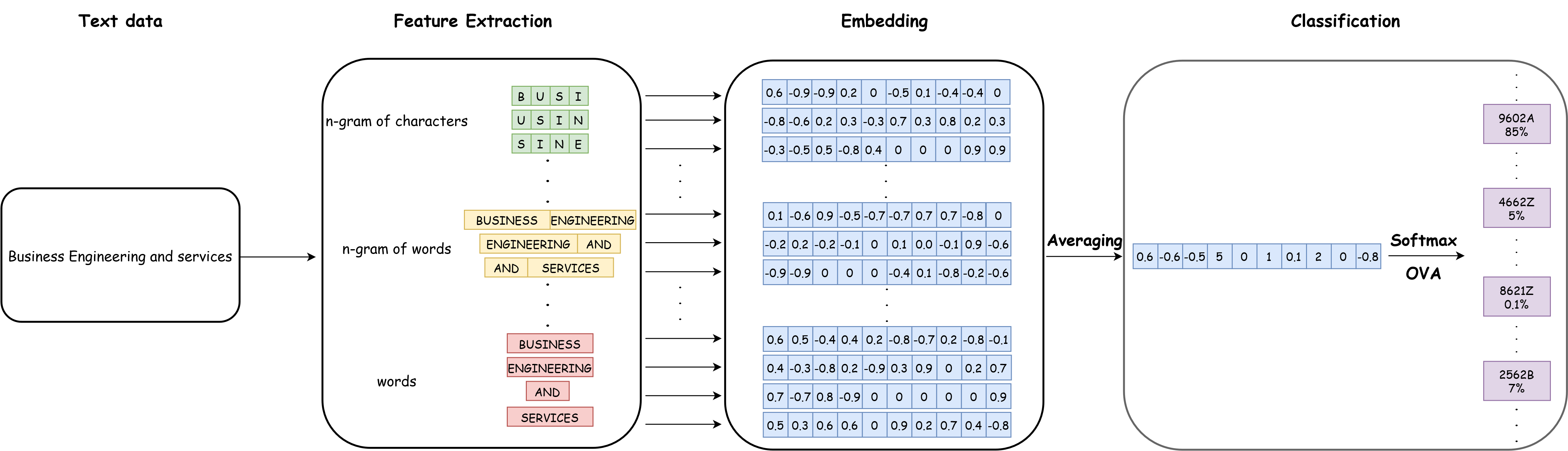
FastText architectureWhat interests us here is the left side of the diagram—“feature extraction”—since the embedding part relates to concepts we will cover in upcoming chapters. In the figure’s example, the text “Business engineering and services” is tokenized into words as we’ve seen earlier. But Fasttext also creates multiple levels of n-grams. For instance, it generates word bigrams: “Business engineering”, “engineering and”, “and services”; and also character four-grams like “busi”, “usin”, and “sine”. Then, Fasttext transforms all these items into numeric vectors. Unlike the term frequency representations we’ve seen, these vectors are not based on corpus frequency (as in document-term matrices) but are word embeddings. We’ll explore this concept in future chapters.
Fasttext is widely used in public statistics, as many textual data sources need to be classified into aggregated nomenclatures.
Here is an example of how such a model can be used for activity classification
Informations additionnelles
NotePython environment
This site was built automatically through a Github action using the Quarto
The environment used to obtain the results is reproducible via uv. The pyproject.toml file used to build this environment is available on the linogaliana/python-datascientist repository
pyproject.toml
[project]
name = "python-datascientist"
version = "0.1.0"
description = "Source code for Lino Galiana's Python for data science course"
readme = "README.md"
requires-python = ">=3.13,<3.14"
dependencies = [
    "altair>=6.0.0",
    "cartiflette",
    "contextily==1.6.2",
    "duckdb>=0.10.1",
    "folium>=0.19.6",
    "gdal==3.11.4",
    "graphviz==0.20.3",
    "great-tables>=0.12.0",
    "gt-extras>=0.0.8",
    "ipykernel>=6.29.5",
    "jupyter>=1.1.1",
    "jupyter-cache>=1.0.0",
    "kaleido>=0.2.1",
    "langchain-community>=0.3.27",
    "loguru==0.7.3",
    "markdown>=3.8",
    "nbclient>=0.10.0",
    "nbformat>=5.10.4",
    "nltk>=3.9.1",
    "pandas>=2.3.3",
    "pip>=25.1.1",
    "plotly>=6.1.2",
    "plotnine>=0.15",
    "polars>=1.8.2",
    "pyarrow>=17.0.0",
    "pynsee>=0.1.8",
    "python-dotenv>=1.0.1",
    "python-frontmatter>=1.1.0",
    "pywaffle>=1.1.1",
    "requests>=2.32.3",
    "scikit-image>=0.24.0",
    "scikit-learn>=1.8.0",
    "scipy>=1.13.0",
    "seaborn>=0.13.2",
    "selenium<4.39.0",
    "spacy>=3.8.4",
    "webdriver-manager>=4.0.2",
    "wordcloud==1.9.3",
]

[tool.uv.sources]
cartiflette = { git = "https://github.com/inseefrlab/cartiflette" }
gdal = [
  { index = "gdal-wheels", marker = "sys_platform == 'linux'" },
  { index = "geospatial_wheels", marker = "sys_platform == 'win32'" },
]

[[tool.uv.index]]
name = "geospatial_wheels"
url = "https://nathanjmcdougall.github.io/geospatial-wheels-index/"
explicit = true

[[tool.uv.index]]
name = "gdal-wheels"
url = "https://gitlab.com/api/v4/projects/61637378/packages/pypi/simple"
explicit = true

[dependency-groups]
dev = [
    "nb-clean>=4.0.1",
]
To use exactly the same environment (version of Python and packages), please refer to the documentation for uv.
NoteFile history
| SHA | Date | Author | Description |
|---|---|---|---|
| d128ca0d | 2025-08-21 22:13:54 | Lino Galiana | Try/Except ici aussi |
| 91431fa2 | 2025-06-09 17:08:00 | Lino Galiana | Improve homepage hero banner (#612) |
| d6b67125 | 2025-05-23 18:03:48 | Lino Galiana | Traduction des chapitres NLP (#603) |
| e1617833 | 2025-05-23 10:08:11 | lgaliana | update uv env & remove discarded code |
| cb655535 | 2024-12-11 08:20:54 | lgaliana | PCA |
| 5df69ccf | 2024-12-05 17:56:47 | lgaliana | up |
| 1b7188a1 | 2024-12-05 13:21:11 | lgaliana | Embedding chapter |
| 5108922f | 2024-08-08 18:43:37 | Lino Galiana | Improve notebook generation and tests on PR (#536) |
| 8d23a533 | 2024-07-10 18:45:54 | Julien PRAMIL | Modifs 02_exoclean.qmd (#523) |
| f32915b9 | 2024-07-09 18:41:00 | Julien PRAMIL | Add badges NLP chapter (#522) |
| 6f2a5658 | 2024-06-16 16:23:01 | linogaliana | Détails tf-idf |
| 8cb248ab | 2024-06-16 16:09:45 | linogaliana | TF-IDF |
| fcdd7b4d | 2024-06-14 15:11:24 | linogaliana | Add spacy corpus |
| 4f41cf6a | 2024-06-14 15:00:41 | Lino Galiana | Une partie sur les sacs de mots plus cohérente (#501) |
| 06d003a1 | 2024-04-23 10:09:22 | Lino Galiana | Continue la restructuration des sous-parties (#492) |
| 005d89b8 | 2023-12-20 17:23:04 | Lino Galiana | Finalise l’affichage des statistiques Git (#478) |
| 3437373a | 2023-12-16 20:11:06 | Lino Galiana | Améliore l’exercice sur le LASSO (#473) |
| 4cd44f35 | 2023-12-11 17:37:50 | Antoine Palazzolo | Relecture NLP (#474) |
| deaafb6f | 2023-12-11 13:44:34 | Thomas Faria | Relecture Thomas partie NLP (#472) |
| 1f23de28 | 2023-12-01 17:25:36 | Lino Galiana | Stockage des images sur S3 (#466) |
| a1ab3d94 | 2023-11-24 10:57:02 | Lino Galiana | Reprise des chapitres NLP (#459) |
| a06a2689 | 2023-11-23 18:23:28 | Antoine Palazzolo | 2ème relectures chapitres ML (#457) |
| 09654c71 | 2023-11-14 15:16:44 | Antoine Palazzolo | Suggestions Git & Visualisation (#449) |
| 889a71ba | 2023-11-10 11:40:51 | Antoine Palazzolo | Modification TP 3 (#443) |
| a7711832 | 2023-10-09 11:27:45 | Antoine Palazzolo | Relecture TD2 par Antoine (#418) |
| 154f09e4 | 2023-09-26 14:59:11 | Antoine Palazzolo | Des typos corrigées par Antoine (#411) |
| a8f90c2f | 2023-08-28 09:26:12 | Lino Galiana | Update featured paths (#396) |
| 80823022 | 2023-08-25 17:48:36 | Lino Galiana | Mise à jour des scripts de construction des notebooks (#395) |
| 3bdf3b06 | 2023-08-25 11:23:02 | Lino Galiana | Simplification de la structure 🤓 (#393) |
| f2905a7d | 2023-08-11 17:24:57 | Lino Galiana | Introduction de la partie NLP (#388) |
| 78ea2cbd | 2023-07-20 20:27:31 | Lino Galiana | Change titles levels (#381) |
| a9b384ed | 2023-07-18 18:07:16 | Lino Galiana | Sépare les notebooks (#373) |
| 29ff3f58 | 2023-07-07 14:17:53 | linogaliana | description everywhere |
| f21a24d3 | 2023-07-02 10:58:15 | Lino Galiana | Pipeline Quarto & Pages 🚀 (#365) |
| 934149d6 | 2023-02-13 11:45:23 | Lino Galiana | get_feature_names is deprecated in scikit 1.0.X versions (#351) |
| 164fa689 | 2022-11-30 09:13:45 | Lino Galiana | Travail partie NLP (#328) |
| f10815b5 | 2022-08-25 16:00:03 | Lino Galiana | Notebooks should now look more beautiful (#260) |
| 494a85ae | 2022-08-05 14:49:56 | Lino Galiana | Images featured ✨ (#252) |
| d201e3cd | 2022-08-03 15:50:34 | Lino Galiana | Pimp la homepage ✨ (#249) |
| 12965bac | 2022-05-25 15:53:27 | Lino Galiana | :launch: Bascule vers quarto (#226) |
| 9c71d6e7 | 2022-03-08 10:34:26 | Lino Galiana | Plus d’éléments sur S3 (#218) |
| 3299f1d9 | 2022-01-08 16:50:11 | Lino Galiana | Clean NLP notebooks (#215) |
| 09b60a18 | 2021-12-21 19:58:58 | Lino Galiana | Relecture suite du NLP (#205) |
| 495599d7 | 2021-12-19 18:33:05 | Lino Galiana | Des éléments supplémentaires dans la partie NLP (#202) |
| 17092b2e | 2021-12-13 09:17:13 | Lino Galiana | Retouches partie NLP (#199) |
| 3c874832 | 2021-12-13 08:46:52 | Lino Galiana | Notebooks NLP update (#198) |
| 2a8809fb | 2021-10-27 12:05:34 | Lino Galiana | Simplification des hooks pour gagner en flexibilité et clarté (#166) |
| 2e4d5862 | 2021-09-02 12:03:39 | Lino Galiana | Simplify badges generation (#130) |
| 49e2826f | 2021-05-13 18:11:20 | Lino Galiana | Corrige quelques images n’apparaissant pas (#108) |
| 4cdb759c | 2021-05-12 10:37:23 | Lino Galiana | :sparkles: :star2: Nouveau thème hugo :snake: :fire: (#105) |
| 7f9f97bc | 2021-04-30 21:44:04 | Lino Galiana | 🐳 + 🐍 New workflow (docker 🐳) and new dataset for modelization (2020 🇺🇸 elections) (#99) |
| d164635d | 2020-12-08 16:22:00 | Lino Galiana | :books: Première partie NLP (#87) |
Footnotes
We use the term bigrams for two-word co-occurrences, trigrams for three-word ones, etc.↩︎
Citation
BibTeX citation:
@book{galiana2025,
  author = {Galiana, Lino},
  title = {Python Pour La Data Science},
  date = {2025},
  url = {https://pythonds.linogaliana.fr/},
  doi = {10.5281/zenodo.8229676},
  langid = {en}
}
For attribution, please cite this work as:
Galiana, Lino. 2025. Python Pour La Data Science. https://doi.org/10.5281/zenodo.8229676.