Python pour la data science

Lino Galiana

doi:10.5281/zenodo.8229676

Warning

Ce chapitre va évoluer prochainement.

If you want to try the examples in this tutorial:

1 Introduction

This page builds on certain aspects presented in the introductory section. We will advance our understanding of NLP issues through language modeling.

We start from the conclusion noted at the end of the previous chapter: frequentist approaches have several shortcomings, such as modeling language based on statistical regularities without considering word or phrase proximity, and difficulty incorporating context.

The aim of this chapter is to address the first of those points. This will serve as an introduction to embeddings, the language representations at the core of modern language models used in everyday tools like DeepL or ChatGPT.

1.1 Data Used

We will continue our exploration of literature using the same three English-language authors:

Edgar Allan Poe (EAP);
HP Lovecraft (HPL);
Mary Wollstonecraft Shelley (MWS).

The dataset is available in a CSV file hosted on Github, and can be directly downloaded from: https://github.com/GU4243-ADS/spring2018-project1-ginnyqg/raw/master/data/spooky.csv.

To explore the topic of embeddings, we will use a language modeling task: predicting the author of a given text. A language model represents a text or language as a probability distribution over terms (usually words).

Sources of Inspiration

This chapter is inspired by several online resources:

A first notebook on Kaggle and a second one;
A Github repository;

1.2 Required Packages

As in the previous section, we need to install specialized NLP libraries along with their dependencies. This tutorial will use several libraries, including some that depend on PyTorch, which is a large framework.

PyTorch on SSPCloud

The following note is only relevant for users of SSPCloud.

The standard Python services on SSPCloud (such as vscode-python and jupyter-python) do not include PyTorch by default. This library is quite large (around 600MB) and requires specific configuration to work seamlessly across different software environments. For ecological sustainability, this enhanced environment is not provided by default. However, when needed, an environment with PyTorch preinstalled is available.

To access it, simply start a vscode-pytorch or jupyter-pytorch service. If you used one of the buttons above, this pre-configured service was automatically launched for you.

!pip install numpy pandas spacy transformers scikit-learn langchain_community

Next, since we will be using the SpaCy library with a corpus of English texts, we need to download the English NLP model. For this, you can refer to the official SpaCy documentation, which is extremely well-designed.

!python -m spacy download en_core_web_sm

2 Data Preparation

We will once again use the spooky dataset:

import pandas as pd

data_url = 'https://github.com/GU4243-ADS/spring2018-project1-ginnyqg/raw/master/data/spooky.csv'
spooky_df = pd.read_csv(data_url)

The dataset pairs each author with a sentence they wrote:

spooky_df.head()

	id	text	author
0	id26305	This process, however, afforded me no means of...	EAP
1	id17569	It never once occurred to me that the fumbling...	HPL
2	id11008	In his left hand was a gold snuff box, from wh...	EAP
3	id27763	How lovely is spring As we looked from Windsor...	MWS
4	id12958	Finding nothing else, not even gold, the Super...	HPL

2.1 Preprocessing

As discussed in the previous chapter, the first step in any work with textual data is often preprocessing, which typically includes tokenization and text cleaning.

Here, we will stick to minimal preprocessing: removing punctuation and stop words (for visualization and count-based vectorization methods).

To begin the cleaning process, we will use the en_core_web_sm model from Spacy

import spacy
nlp = spacy.load('en_core_web_sm')

We will use a spacy pipe that automates and parallelizes a number of operations. Pipes in NLP are similar to scikit pipelines or pandas pipes. They are well-suited tools for industrializing various preprocessing tasks:

Preprocessing de la base textuelle

from typing import List
import spacy

def clean_docs(
    texts: List[str],
    remove_stopwords: bool = False,
    n_process: int = 4,
    remove_punctuation: bool = True
) -> List[str]:
    """
    Cleans a list of text documents by tokenizing, optionally removing stopwords, and optionally removing punctuation.

    Parameters:
        texts (List[str]): List of text documents to clean.
        remove_stopwords (bool): Whether to remove stopwords. Default is False.
        n_process (int): Number of processes to use for processing. Default is 4.
        remove_punctuation (bool): Whether to remove punctuation. Default is True.

    Returns:
        List[str]: List of cleaned text documents.
    """
    # Load spacy's nlp model
    docs = nlp.pipe(
        texts,
        n_process=n_process,
        disable=['parser', 'ner', 'lemmatizer', 'textcat']
    )

    # Pre-load stopwords for faster checking
    stopwords = set(nlp.Defaults.stop_words)

    # Process documents
    docs_cleaned = (
        ' '.join(
            tok.text.lower().strip()
            for tok in doc
            if (not remove_punctuation or not tok.is_punct) and
               (not remove_stopwords or tok.text.lower() not in stopwords)
        )
        for doc in docs
    )

    return list(docs_cleaned)

We apply the clean_docs function to our pandas column. Since pandas.Series are iterable, they behave like lists and work very well with our spacy pipe.

spooky_df['text_clean'] = clean_docs(spooky_df['text'])

spooky_df.head()

	id	text	author	text_clean
0	id26305	This process, however, afforded me no means of...	EAP	this process however afforded me no means of a...
1	id17569	It never once occurred to me that the fumbling...	HPL	it never once occurred to me that the fumbling...
2	id11008	In his left hand was a gold snuff box, from wh...	EAP	in his left hand was a gold snuff box from whi...
3	id27763	How lovely is spring As we looked from Windsor...	MWS	how lovely is spring as we looked from windsor...
4	id12958	Finding nothing else, not even gold, the Super...	HPL	finding nothing else not even gold the superin...

2.2 Encoding the Target Variable

We perform a simple encoding of the target variable: there are three categories (authors), represented by integers 0, 1, and 2. For this, we use Scikit’s LabelEncoder, previously introduced in the modeling section. We will use the fit_transform method, which conveniently combines fitting (i.e., creating a mapping between numerical values and labels) and transforming the same column in one step.

We can check the classes of our LabelEncoder:

array(['EAP', 'HPL', 'MWS'], dtype=object)

2.3 Creating the Training and Test Sets

We set aside a test sample (20%) before performing any analysis (even descriptive). This ensures a rigorous evaluation of our models at the end, since these data will never have been seen during training.

Our initial dataset is not balanced—some authors have more texts than others. To ensure fair evaluation of our model, we will stratify the sampling so that the training and test sets contain a similar distribution of authors.

from sklearn.model_selection import train_test_split

y = spooky_df["author"]
X = spooky_df['text_clean']
X_train, X_test, y_train, y_test = train_test_split(
    X, y, test_size=0.2, stratify=y, random_state=42
)

Preview of the first element in X_train:

'this process however afforded me no means of ascertaining the dimensions of my dungeon as i might make its circuit and return to the point whence i set out without being aware of the fact so perfectly uniform seemed the wall'

3 Vectorization Using the Bag of Words Approach

Representing our texts as a bag of words allows us to vectorize the corpus and thus obtain a numerical representation of each text. From there, we can perform various types of modeling tasks.

Let’s define our vector representation using TF-IDF with Scikit:

from sklearn.feature_extraction.text import TfidfVectorizer
from sklearn.pipeline import Pipeline

pipeline_tfidf = Pipeline([
    ('tfidf', TfidfVectorizer(max_features=10000)),
])
pipeline_tfidf

Pipeline(steps=[('tfidf', TfidfVectorizer(max_features=10000))])

In a Jupyter environment, please rerun this cell to show the HTML representation or trust the notebook.
On GitHub, the HTML representation is unable to render, please try loading this page with nbviewer.org.

Let’s go ahead and train our model to vectorize the text using the TF-IDF method. At this stage, we are not yet concerned with evaluation, so we will train on the entire dataset, not just X_train.

pipeline_tfidf.fit(spooky_df['text_clean'])

Pipeline(steps=[('tfidf', TfidfVectorizer(max_features=10000))])

In a Jupyter environment, please rerun this cell to show the HTML representation or trust the notebook.
On GitHub, the HTML representation is unable to render, please try loading this page with nbviewer.org.

3.1 Finding the Most Similar Text

First, we can look for the text that is closest—according to TF-IDF similarity—to a given sentence. Let’s take the following example:

text = "He was afraid by Frankenstein monster"

How can we find the text most similar to this one? We need to transform our sentence into the same vector representation, then compare it to the other texts using that same form.

This is essentially an information retrieval task—a classic NLP use case—implemented, for example, by search engines. Since the term “Frankenstein” is quite distinctive, we should be able to identify similarities with other texts written by Mary Shelley using TF-IDF.

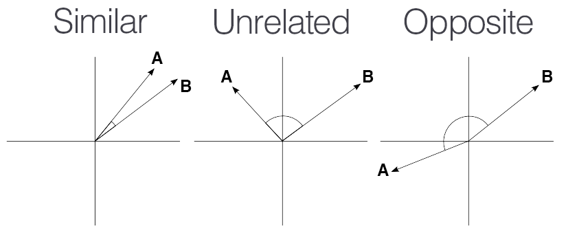
A metric commonly used to compare vectors is cosine similarity. This is a central measure in modern NLP. While it is more meaningful with dense vectors (which we’ll explore soon), it still provides a useful exercise for understanding similarity between two vectors, even when those vectors are sparse, as in the bag-of-words approach.

If each dimension of a vector represents a direction, cosine similarity measures the angle between two vectors. The smaller the angle, the closer the vectors.

3.1.1 With `Scikit-Learn`

Exercise 1: Similarity Search with TF-IDF

Use the transform method to vectorize the entire training corpus.
Assuming your vectorized training set is named X_train_tfidf, you can convert it to a DataFrame with the following command:

X_train_tfidf = pd.DataFrame(
    X_train_tfidf.todense(), columns=pipeline_tfidf.get_feature_names_out()
)

Use Scikit’s cosine_similarity method to compute cosine similarity between your vectorized text and the training corpus using this code:

import numpy as np
from sklearn.metrics.pairwise import cosine_similarity

cosine_similarities = cosine_similarity(
    X_train_tfidf,
    pipeline_tfidf.transform([text])
).flatten()

top_4_indices = np.argsort(cosine_similarities)[-4:][::-1]  # Descending sort
top_4_similarities = cosine_similarities[top_4_indices]

Retrieve the corresponding documents. Are you satisfied with the result? Do you understand what happened?

A l’issue de l’exercice, les 4 textes les plus similaires sont:

	text	author	score
8181	Listen to me, Frankenstein.	MWS	0.402964
8606	He was gazing at me gaspingly and fascinatedly...	HPL	0.330177
14550	The light is dimmer and the gods are afraid. . .	HPL	0.314670
11366	I screamed aloud that I was not afraid; that I...	HPL	0.311235

3.1.2 With `Langchain`

This approach to computing text similarity is rather tedious with Scikit. With the rapid development of Python applications leveraging language models, a rich ecosystem has emerged to make these tasks achievable in just a few lines of code.

Among the most valuable tools is Langchain, a high-level Python ecosystem for building production-ready pipelines using textual data.

We will proceed here in two steps:

Create a retriever, which involves vectorizing our corpus (texts from the three authors) using TF-IDF and storing it in a vector database.
Vectorize our search query (text, created earlier) on the fly and retrieve its closest match from the vector database.

Vectorizing our corpus is very straightforward using Langchain, as Scikit’s TfidfVectorizer is wrapped in a dedicated module provided by Langchain.

from langchain_community.retrievers import TFIDFRetriever
from langchain_community.document_loaders import DataFrameLoader

loader = DataFrameLoader(spooky_df, page_content_column="text_clean")

retriever = TFIDFRetriever.from_documents(
    loader.load()
)

This retriever object serves as an entry point to our corpus. Langchain is particularly valuable in NLP projects because it provides standardized entry points, allowing you to easily switch out vectorizers without needing to change how the results are used at the end of the pipeline.

The invoke method is used to find the most similar vectors to our search query:

retriever.invoke(text)

[Document(metadata={'id': 'id12587', 'text': 'Listen to me, Frankenstein.', 'author': 'MWS', 'author_encoded': 2}, page_content='listen to me frankenstein'),
 Document(metadata={'id': 'id09284', 'text': 'I screamed aloud that I was not afraid; that I never could be afraid; and others screamed with me for solace.', 'author': 'HPL', 'author_encoded': 1}, page_content='i screamed aloud that i was not afraid that i never could be afraid and others screamed with me for solace'),
 Document(metadata={'id': 'id09797', 'text': 'It seemed to be a sort of monster, or symbol representing a monster, of a form which only a diseased fancy could conceive.', 'author': 'HPL', 'author_encoded': 1}, page_content='it seemed to be a sort of monster or symbol representing a monster of a form which only a diseased fancy could conceive'),
 Document(metadata={'id': 'id10816', 'text': 'And, as I have implied, it was not of the dead man himself that I became afraid.', 'author': 'HPL', 'author_encoded': 1}, page_content='and as i have implied it was not of the dead man himself that i became afraid')]

The output is a Langchain object, which is not convenient for our purposes here. We convert it into a DataFrame:

documents = []
for best_echoes in retriever.invoke(text):
    documents += [{**best_echoes.metadata, **{"text_clean": best_echoes.page_content}}]

documents = pd.DataFrame(documents)

We can add the similarity score column to this DataFrame:

We do indeed retrieve the same documents:

	id	text	author	author_encoded	text_clean	score
0	id12587	Listen to me, Frankenstein.	MWS	2	listen to me frankenstein	0.402964
1	id09284	I screamed aloud that I was not afraid; that I...	HPL	1	i screamed aloud that i was not afraid that i ...	0.311235
2	id09797	It seemed to be a sort of monster, or symbol r...	HPL	1	it seemed to be a sort of monster or symbol re...	0.295587
3	id10816	And, as I have implied, it was not of the dead...	HPL	1	and as i have implied it was not of the dead m...	0.261818

The BM25 Metric

BM25 is a probabilistic relevance-based information retrieval model, similar to TF-IDF. It is commonly used in search engines to rank documents relative to a query.

BM25 combines term frequency (TF), inverse document frequency (IDF), and a normalization based on document length. In other words, it improves on TF-IDF by adjusting scores based on string length to avoid overemphasizing longer documents.

BM25 performs particularly well in environments where documents vary in length and content. This is why search engines such as Elasticsearch have made it a cornerstone of their search mechanisms.

Why aren’t all results relevant? We can anticipate several reasons.

The first hypothesis is that we’re training our vectorizer on a biased corpus. While “Frankenstein” is a rare term, it appears more frequently in our dataset than in general English usage. The inverse document frequency is thus biased against the term: its appearance should be a much stronger indicator that the text belongs to Mary Shelley. While addressing this might slightly improve relevance, it’s not the core issue.

The frequentist approach assumes all terms are equally distinct. A sentence containing the word “creature” won’t get a higher score when searching for “monster”. Again, we’ve treated our corpus as a bag where words are independent—there’s no increased likelihood of encountering “Frankenstein” after “doctor”. These limitations point us toward the topic of embeddings. Even though the frequentist method may seem a bit old school, it’s not useless and often provides a “tough to beat baseline.” In fields like information extraction from short texts, where every term carries strong signal, this approach is often effective.

3.2 Finding the Closest Author: An Introduction to the Naive Bayes Classifier

Before diving into embeddings, let’s explore a slightly different use case within our probabilistic framework. Suppose we want to predict the author of a given text. If our previous intuition holds—certain words are more likely to appear in texts by specific authors—then we can train an automatic classification algorithm to predict the author based on the text.

The most natural method for this task is the Naive Bayes classifier. This model is a perfect fit for the frequentist approach we’ve used so far, as it relies on the probabilities of word occurrences per author.

The Naive Bayes classifier applies a decision rule: it selects the most probable class given the observed structure of the document—i.e., the words that appear in it.

In other words, we choose the class \(\widehat{c}\) that is most probable given the terms in document \(d\).

\[ \widehat{c} = \arg \max_{c \in \mathcal{C}} \mathbb{P}(c|d) = \arg \max_{c \in \mathcal{C}} \frac{ \mathbb{P}(d|c)\mathbb{P}(c)}{\mathbb{P}(d)} \tag{3.1}\]

As is common in Bayesian estimation, we can ignore constant terms such as \(\mathbb{P}(d)\). The definition of the predicted class can thus be reformulated as follows:

\[ \widehat{c} = \arg \max_{c \in \mathcal{C}} \mathbb{P}(d|c)\mathbb{P}(c) \tag{3.2}\]

The bag-of-words assumption comes into play here. A document \(d\) is considered a collection of words \(w_i\), where word order is irrelevant. In other words, we can build a model based on individual words without involving conditional probabilities related to their order. The second strong assumption is the naive assumption from which the method gets its name: the probability of drawing a word depends only on the category \(c\) to which the document belongs. In other words, a document is treated as a sequence of independent word draws, where the probability depends solely on the author.

As explained in the dedicated box, under these assumptions, the classifier can be rewritten in the following form

\[ \widehat{c} = \arg \max_{c \in \mathcal{C}} \mathbb{P}(c)\prod_{w \in \mathcal{W}}{\mathbb{P}(w|c)} \]

where \(\mathcal{W}\) is the set of words in the corpus (our vocabulary).

Empirically, this is a supervised learning task where the label is the document class and the features are our vectorized words. In practice, the probabilities are estimated from word counts in the corpus and the distribution of document types.

While it is possible to compute all these quantities manually, Scikit makes it easy to implement a Naive Bayes estimator after vectorizing the corpus, as shown in the next exercise. However, this may introduce a practical issue: ideally, the test set should not contain new words that were not in the training set, since these new dimensions did not exist during training. In practice, the most common solution is the one adopted here: these words are ignored.

Exercise 2: The Naive Bayes Classifier

Starting from the previous example, define a pipeline that vectorizes each document (using CountVectorizer instead of TFIDFVectorizer) and performs prediction using a Naive Bayes model.
Train this model and make predictions on the test set.
Evaluate the performance of your model.
Make a prediction for the sentence we previously stored in the text variable. Do you get the expected result?
Examine the predicted probabilities (using the predict_proba method).

from sklearn.feature_extraction.text import CountVectorizer
from sklearn.naive_bayes import MultinomialNB

pipeline = Pipeline([
    ('vectorizer', CountVectorizer()),
    ('classifier', MultinomialNB())
])

# Train the pipeline on the training data
pipeline.fit(X_train, y_train)

Pipeline(steps=[('vectorizer', CountVectorizer()),
                ('classifier', MultinomialNB())])

In a Jupyter environment, please rerun this cell to show the HTML representation or trust the notebook.
On GitHub, the HTML representation is unable to render, please try loading this page with nbviewer.org.

We obtain a satisfactory accuracy:

Précision: 0.8429519918283963

The breakdown of performance metrics is as follows:

              precision    recall  f1-score   support

         EAP       0.85      0.85      0.85      1580
         HPL       0.87      0.82      0.84      1127
         MWS       0.81      0.86      0.83      1209

    accuracy                           0.84      3916
   macro avg       0.84      0.84      0.84      3916
weighted avg       0.84      0.84      0.84      3916

Unsurprisingly, we get Mary Shelley as the predicted author:

np.str_('MWS')

Finally, when examining the predicted probabilities (question 5), we see that the prediction is very confident:

	author	proba
0	EAP	0.001675
1	HPL	0.084844
2	MWS	0.913481

Understanding the logic of the naive Bayes classifier

Suppose we are in a classification problem with classes \((c_1,...,c_K)\) (set denoted \(\mathcal{C}\)). Placing ourselves within the bag-of-words framework, we can ignore the positions of words in documents, which would greatly complicate the writing of our equations.

The equation Equation 3.2 can be rewritten

\[ \widehat{c} = \arg \max_{c \in \mathcal{C}} \mathbb{P}(w_1, ..., w_n|c)\mathbb{P}(c) \]

In the Bayesian world, we call \(\mathbb{P}(w_1, ..., w_n|c)\) the likelihood and \(\mathbb{P}(c)\) the prior.

The naive Bayes assumption allows us to treat a document as a sequence of random draws whose probabilities depend only on the category. In this case, drawing a sentence is a sequence of word draws and the compound probability is therefore

\[ \mathbb{P}(w_1, ..., w_n|c) = \prod_{i=1}^n \mathbb{P}(w_i|c) \]

For example, simplifying to two classes, if the probabilities are those from Table 3.1, the sentence “afraid by Doctor Frankenstein” will have a little less than 1% chance (0.8%) of being written if the author is Mary Shelley but will be even less likely with Lovecraft (0.006%) because while “afraid” is very probable with him, Frankenstein is a rare event that makes this word composition unlikely.

Table 3.1: Fictional example of drawing probabilities

Word (\(w_i\))	Probability for Mary Shelley	Probability for Lovecraft
Afraid	0.1	0.6
By	0.2	0.2
Doctor	0.2	0.05
Frankenstein	0.2	0.01

By combining these different equations, we get

\[ \widehat{c} = \arg \max_{c \in \mathcal{C}} \mathbb{P}(c)\prod_{w \in \mathcal{W}}{\mathbb{P}(w|c)} \]

The empirical counterpart of \(\mathbb{P}(c)\) is quite obvious: the observed frequency of each category (the authors) in our corpus. In other words,

\[ \widehat{\mathbb{P}(c)} = \frac{n_c}{n_{doc}} \]

What is the empirical counterpart of \(\mathbb{P}(w_i|c)\)? It is the frequency of appearance of the word in question for the author. To calculate it, we simply count the number of times it appears for the author and divide by the number of words by the author.

4 The Word2Vec model, a more synthetic representation

4.1 Towards a more synthetic representation of language

The vector representation resulting from the bag of words approach is not very synthetic or stable and is quite crude.

If we have a small corpus, we will have problems extrapolating since new texts are very likely to bring new words, which are new feature dimensions that were not present in the training corpus. This is conceptually a problem since machine learning algorithms are not intended to predict on characteristics they have not been trained on¹.

Conversely, the more text we have in a corpus, the larger our vector representation will be. For example, if your bag of words has seen the entire French vocabulary, which is 60,000 words according to the French Academy (estimates being 200,000 for the English language), this results in vectors of considerable size. However, the diversity of texts is, in practice, much lower: common use of French requires around 3,000 words and most texts, especially if they are short, do not use such a complete vocabulary. This therefore implies very sparse vectors, with many 0s.

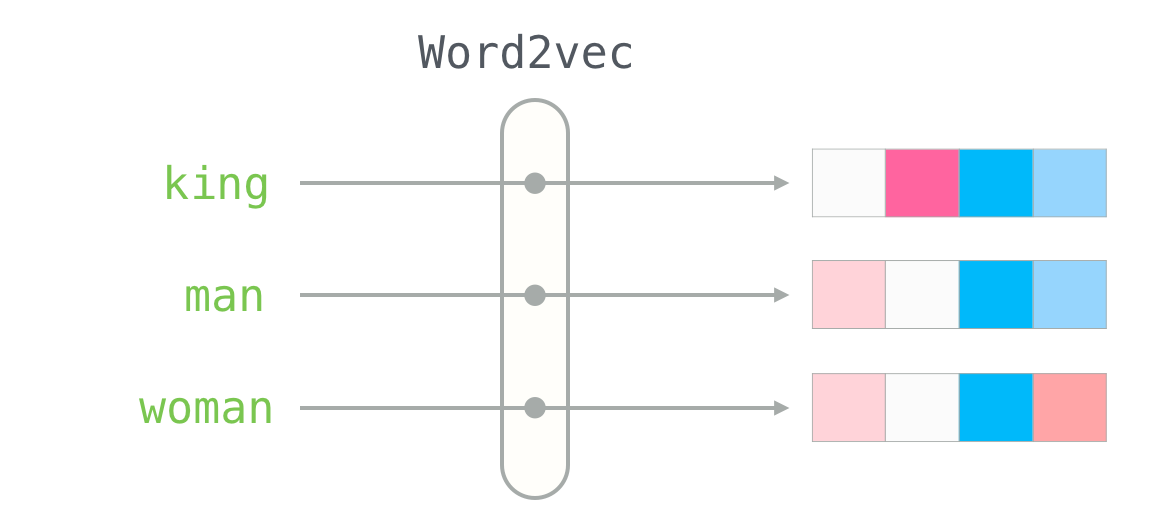
Vectorization according to this approach is therefore inefficient; the signal is poorly compressed. Dense representations, that is, of smaller dimension but all carrying information, seem more adequate to be able to generalize our language modeling. The algorithm that made this approach famous is the Word2Vec model, in some ways the first common ancestor of modern LLMs. The vector representation of Word2Vec is quite synthetic: the dimension of these embeddings is between 100 and 300.

4.2 Semantic relationships between terms

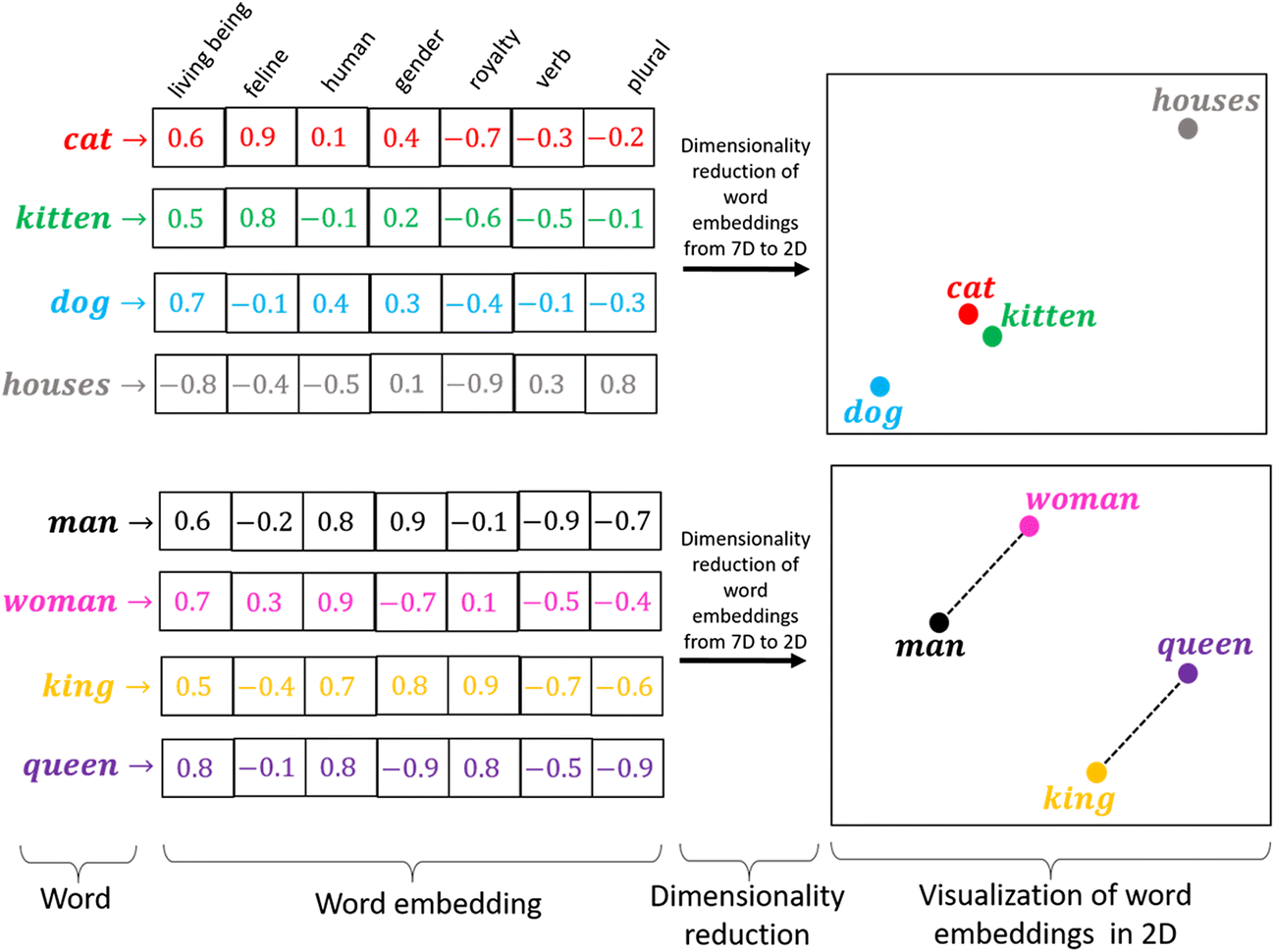
This dense representation will represent a solution to a limitation of the bag of words approach that we have mentioned multiple times. Each of these dimensions will represent a latent factor, that is, an unobserved variable, in the same way as principal components produced by a PCA. These latent dimensions can be interpreted as “fundamental” dimensions of language.

Illustration of the principle of Word2Vec representation (source: Jay Alammar)

For example, a human knows that a document containing the word “King” and another document containing the word “Queen” are very likely to address similar subjects. A well-trained Word2Vec model will capture that there exists a latent factor of type “royalty” and the similarity between the vectors associated with the two words will be strong.

The magic goes even further: the model will also capture that there exists a latent factor of type “gender”, and will allow the construction of a semantic space in which arithmetic relationships between vectors make sense. For example,

\[ \text{king} - \text{man} + \text{woman} ≈ \text{queen} \]

or, to revisit the example from the original Word2Vec paper (Mikolov 2013),

\[ \text{Paris} - \text{France} + \text{Italy} ≈ \text{Rome} \]

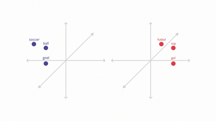
Illustration of lexical embedding. Source: Blog post Word Embedding: Basics

Another “miracle” of this approach is that it allows a form of transfer between languages. Since semantic relationships can be similar across languages, many common words can be mapped between languages if they share a common base (such as Western languages). This concept is the foundation of automatic translators and multilingual AI systems.

Example of translation between two vector representations. Source: Meta

4.3 How are these models trained?

These models are trained from a prediction task solved by a simple neural network, generally with a reinforcement approach.

The fundamental idea is that the meaning of a word is understood by looking at words that frequently appear in its neighborhood. For a given word, we will therefore try to predict the words that appear in a window around the target word.

By repeating this task many times and on a sufficiently varied corpus, we finally obtain embeddings for each word in the vocabulary, which present the properties discussed previously. The collection of Wikipedia articles is one of the preferred corpora for people who have built lexical embeddings. It indeed contains complete sentences, unlike information from social media comments, and proposes interesting connections between people, places, etc.

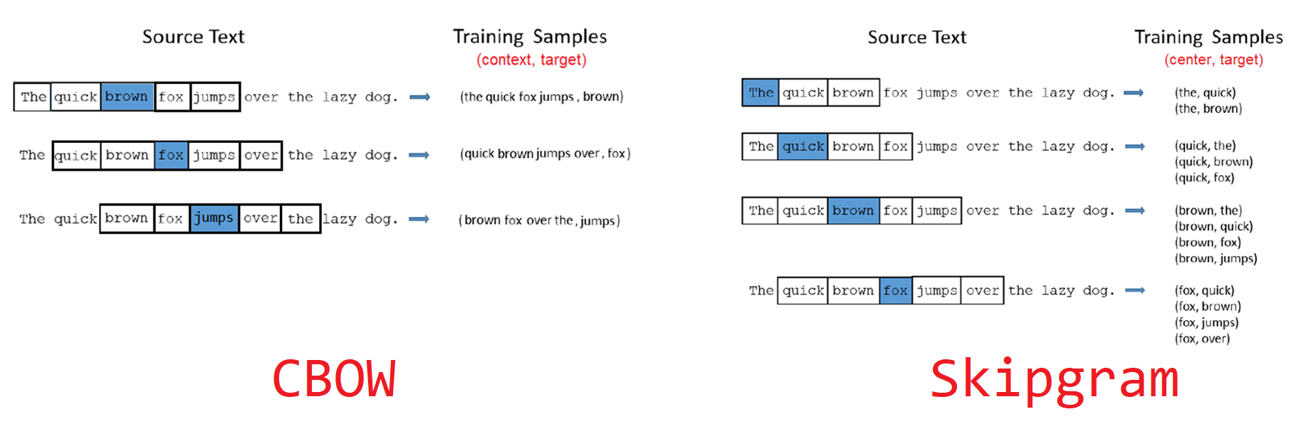
The context of a word is defined by a fixed-size window around this word. The window size is a parameter of the embedding construction. The corpus provides a large set of word-context examples, which can be used to train a neural network.

More precisely, there are two approaches, whose details we will not develop:

Continuous bag of words (CBOW), where the model is trained to predict a word from its context;
Skip-gram, where the model attempts to predict the context from a single word.

Illustration of the difference between CBOW and Skip-gram approaches

4.4 Related models

Several models have a direct lineage with the Word2Vec model although they distinguish themselves by the nature of the architecture used.

This is the case, for example, of the GloVe model, developed in 2014 at Stanford, which does not rely on neural networks but on the construction of a large word co-occurrence matrix. For each word, the task is to calculate the frequencies of appearance of other words in a fixed-size window around it. The obtained co-occurrence matrix is then factorized by a singular value decomposition.

The FastText model, developed in 2016 by a Facebook team, works similarly to Word2Vec but particularly distinguishes itself on two points:

In addition to the words themselves, the model learns representations for character n-grams (character subsequences of size \(n\), for example “tar”, “art” and “rte” are the trigrams of the word “tarte”), which makes it particularly robust to spelling variations;
The model has been optimized so that its training is particularly fast.

The FastText model is particularly effective for automatic classification problems. INSEE uses it for example for several models of classification of textual labels in nomenclatures.

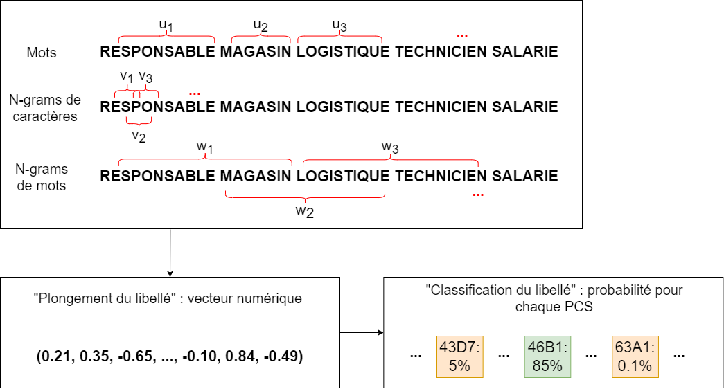
Here is an example of an automated profession classification project in the typology of activity nomenclatures (PCS) based on a model trained by the Fasttext library:

viewof activite = Inputs.text(
  {label: '', value: 'data scientist', width: 800}
)

d3.json(urlApe).then(res => {
  var IC, results;

  ({ IC, ...results } = res);

  IC = parseFloat(IC);

  const rows = Object.values(results).map(obj => {
    return `
    <tr>
      <td>${obj.code} | ${obj.libelle}</td>
      <td>${obj.probabilite.toFixed(3)}</td>
    </tr>
  `;
  }).join('');

  const confidenceRow = `<tr>
    <td colspan="2" style="text-align:left; "><em>Indice de confiance : ${IC.toFixed(3)}</em></td>
  </tr>`;

  const tableHTML = html`
  <table>
    <caption>
      Prédiction de l'activité
    </caption>
    <tr>
      <th style="text-align:center;">Libellé (NA2008)</th>
      <th>Probabilité</th>
    </tr>
      ${rows}
      ${confidenceRow}
  </table>`;

  // Now you can use the tableHTML as needed, for example, inserting it into the DOM.
  // For example, assuming you have a container with the id "tableContainer":
  return tableHTML;
});

activite_debounce = debounce(viewof activite, 2000)
urlApe = `https://codification-ape-test.lab.sspcloud.fr/predict?nb_echos_max=3&prob_min=0&text_feature=${activite_debounce}`

import {debounce} from "@mbostock/debouncing-input"

These models are inheritors of Word2Vec in the sense that they adopt a dense, low-dimensional vector representation of textual documents. Word2Vec remains a model that inherits from the bag-of-words logic. The representation of a sentence or document is a form of average of the representations of the words that compose them.

Since 2013, several revolutions have led to enriching language models to go beyond a word-by-word representation of these. Much more complex architectures to represent not only words in the form of embeddings but also sentences and documents are now at work and can be linked to the revolution of transformer architectures.

5 Transformers: a richer representation of language

While the Word2Vec model is trained contextually, its purpose is to give a vector representation of a word in an absolute manner, independent of context. For example, the term “bank” will have exactly the same vector representation whether it appears in the sentence “She runs towards the sandbank” or “He’s waiting for you on a bench in the park”. This is a major limitation of this type of approach and we can well imagine the importance of context for language interpretation.

The objective of transformer architectures is to enable contextual vector representations. In other words, a word will have several vector representations, depending on its context of occurrence. These models rely on the attention mechanism (Vaswani 2017). Before this approach, when a model learned to vectorize a text and reached the nth word, the only memory it kept was that of the previous word. By recurrence, this meant it kept a memory of previous words but this tended to dissipate. Consequently, for a word appearing far in the sentence, it was likely that the context from the beginning of the sentence was forgotten. In other words, in the sentence “at the beach, he was going to explore the bank”, it was very likely that upon reaching the word “bank”, the model had forgotten the beginning of the sentence which was nevertheless important for interpretation.

The objective of the attention mechanism is to create an internal memory in the model allowing, for any word in a text, to keep track of other words. Of course, not all are relevant for interpreting the text but this avoids forgetting those that are important. The main innovation of recent years in NLP has been to manage to create large-scale attention mechanisms without making the models intractable. The context windows of the most performant models are becoming immense. For example, the Llama 3.1 model (made public by Meta in July 2024) offers a context window of 128,000 tokens, or about 96,000 words, the equivalent of Tolkien’s Hobbit. In other words, to deduce the subtlety of a word’s meaning, this model can browse through a context as long as a novel of about 300 pages.

The two models that marked their era in the field are the BERT models developed in 2018 by Google (which was already behind Word2Vec) and the first version of the well-known GPT from OpenAI, which, in 2017, was the first pre-trained model based on the transformer architecture. These two transformer families differ in how they integrate context to make a prediction. GPT is an autoregressive model, therefore only considers the tokens before the one we want to predict. BERT uses the tokens to the left and right to infer context. These two major trained language models are trained by self-reinforcement, mainly on next token prediction tasks (Face 2022). Since the success of ChatGPT, the new GPT models (from version 3 onwards) are no longer open source. To use them, one must therefore go through OpenAI’s APIs. There are nevertheless many alternatives whose weights are open, if not open source², which allow using these LLMs through Python, notably through the transformers library developed by Hugging Face.

When working with small-sized corpora, it’s generally a bad idea to train your own model from scratch. Fortunately, models pre-trained on very large corpora are available. They allow for transfer learning, that is, to benefit from the performance of a model that has been trained on another task or on another corpus.

Exercise 3

Repeat a train/test split with 500 random lines
Import the all-MiniLM-L6-v2 model with the sentence transformers package. Encode X_train and X_test.
Perform a classification using a simple method, such as CVS, based on the embeddings produced in the previous question. As the training set is small, you can perform cross-validation.
Understand why the performance is worse than that of Bayes’ naive classifier.

Answer to question 1:

random_rows = spooky_df.sample(500)
y = random_rows["author"]
X = random_rows['text']

X_train, X_test, y_train, y_test = train_test_split(
    X, y, test_size=0.2, stratify=y, random_state=42
)

Réponse à la question 2:

from sentence_transformers import SentenceTransformer
from sklearn.svm import LinearSVC

model = SentenceTransformer(
    "all-MiniLM-L6-v2", model_kwargs={"torch_dtype": "float16"}
)

X_train_vectors = model.encode(X_train.values)
X_test_vectors = model.encode(X_test.values)

Answer to question 3:

from sklearn.model_selection import cross_val_score

clf = LinearSVC(max_iter=10000, C=0.1, dual="auto")

scores = cross_val_score(
    clf, X_train_vectors, y_train,
    cv=4, scoring='f1_micro', n_jobs=4
)

print(f"CV scores {scores}")
print(f"Mean F1 {np.mean(scores)}")

But why, with a very complicated method, can’t we beat a very simple one?

There are several possible reasons:

the TF-IDF is a simple model, but it still performs very well (this is known as a ‘tough-to-beat baseline’).
the classification of authors is a very specific and arduous task, which does not do justice to the embeddings. As we said earlier, the latter are particularly relevant when it comes to semantic similarity between texts (clustering, etc.).

In the case of our classification task, it is likely that certain words (character names, place names) are sufficient to classify in a relevant way, This is not captured by embeddings, which give all words the same importance.

Informations additionnelles

environment files have been tested on.

Latest built version: 2025-05-26

Python version used:

'3.12.6 | packaged by conda-forge | (main, Sep 30 2024, 18:08:52) [GCC 13.3.0]'

Package	Version
affine	2.4.0
aiobotocore	2.15.1
aiohappyeyeballs	2.4.3
aiohttp	3.10.8
aioitertools	0.12.0
aiosignal	1.3.1
alembic	1.13.3
altair	5.4.1
aniso8601	9.0.1
annotated-types	0.7.0
anyio	4.9.0
appdirs	1.4.4
archspec	0.2.3
asttokens	2.4.1
attrs	24.2.0
babel	2.17.0
bcrypt	4.2.0
beautifulsoup4	4.12.3
black	24.8.0
blinker	1.8.2
blis	1.3.0
bokeh	3.5.2
boltons	24.0.0
boto3	1.35.23
botocore	1.35.23
branca	0.7.2
Brotli	1.1.0
bs4	0.0.2
cachetools	5.5.0
cartiflette	0.1.9
Cartopy	0.24.1
catalogue	2.0.10
cattrs	24.1.3
certifi	2025.4.26
cffi	1.17.1
charset-normalizer	3.3.2
chromedriver-autoinstaller	0.6.4
click	8.1.7
click-plugins	1.1.1
cligj	0.7.2
cloudpathlib	0.21.1
cloudpickle	3.0.0
colorama	0.4.6
comm	0.2.2
commonmark	0.9.1
conda	24.9.1
conda-libmamba-solver	24.7.0
conda-package-handling	2.3.0
conda_package_streaming	0.10.0
confection	0.1.5
contextily	1.6.2
contourpy	1.3.0
cryptography	43.0.1
cycler	0.12.1
cymem	2.0.11
cytoolz	1.0.0
dask	2024.9.1
dask-expr	1.1.15
databricks-sdk	0.33.0
dataclasses-json	0.6.7
debugpy	1.8.6
decorator	5.1.1
Deprecated	1.2.14
diskcache	5.6.3
distributed	2024.9.1
distro	1.9.0
docker	7.1.0
duckdb	1.1.1
en_core_web_sm	3.8.0
entrypoints	0.4
et_xmlfile	2.0.0
exceptiongroup	1.2.2
executing	2.1.0
fastexcel	0.14.0
fastjsonschema	2.21.1
fiona	1.10.1
Flask	3.0.3
folium	0.19.6
fontawesomefree	6.6.0
fonttools	4.54.1
fr_core_news_sm	3.8.0
frozendict	2.4.4
frozenlist	1.4.1
fsspec	2024.9.0
geographiclib	2.0
geopandas	1.0.1
geoplot	0.5.1
geopy	2.4.1
gitdb	4.0.11
GitPython	3.1.43
google-auth	2.35.0
graphene	3.3
graphql-core	3.2.4
graphql-relay	3.2.0
graphviz	0.20.3
great-tables	0.12.0
greenlet	3.1.1
gunicorn	22.0.0
h11	0.16.0
h2	4.1.0
hpack	4.0.0
htmltools	0.6.0
httpcore	1.0.9
httpx	0.28.1
httpx-sse	0.4.0
hyperframe	6.0.1
idna	3.10
imageio	2.37.0
importlib_metadata	8.5.0
importlib_resources	6.4.5
inflate64	1.0.1
ipykernel	6.29.5
ipython	8.28.0
itsdangerous	2.2.0
jedi	0.19.1
Jinja2	3.1.4
jmespath	1.0.1
joblib	1.4.2
jsonpatch	1.33
jsonpointer	3.0.0
jsonschema	4.23.0
jsonschema-specifications	2025.4.1
jupyter-cache	1.0.0
jupyter_client	8.6.3
jupyter_core	5.7.2
kaleido	0.2.1
kiwisolver	1.4.7
langchain	0.3.25
langchain-community	0.3.9
langchain-core	0.3.61
langchain-text-splitters	0.3.8
langcodes	3.5.0
langsmith	0.1.147
language_data	1.3.0
lazy_loader	0.4
libmambapy	1.5.9
locket	1.0.0
loguru	0.7.3
lxml	5.4.0
lz4	4.3.3
Mako	1.3.5
mamba	1.5.9
mapclassify	2.8.1
marisa-trie	1.2.1
Markdown	3.6
markdown-it-py	3.0.0
MarkupSafe	2.1.5
marshmallow	3.26.1
matplotlib	3.9.2
matplotlib-inline	0.1.7
mdurl	0.1.2
menuinst	2.1.2
mercantile	1.2.1
mizani	0.11.4
mlflow	2.16.2
mlflow-skinny	2.16.2
msgpack	1.1.0
multidict	6.1.0
multivolumefile	0.2.3
munkres	1.1.4
murmurhash	1.0.13
mypy_extensions	1.1.0
narwhals	1.41.0
nbclient	0.10.0
nbformat	5.10.4
nest_asyncio	1.6.0
networkx	3.3
nltk	3.9.1
numpy	2.1.2
opencv-python-headless	4.10.0.84
openpyxl	3.1.5
opentelemetry-api	1.16.0
opentelemetry-sdk	1.16.0
opentelemetry-semantic-conventions	0.37b0
orjson	3.10.18
outcome	1.3.0.post0
OWSLib	0.33.0
packaging	24.1
pandas	2.2.3
paramiko	3.5.0
parso	0.8.4
partd	1.4.2
pathspec	0.12.1
patsy	0.5.6
Pebble	5.1.1
pexpect	4.9.0
pickleshare	0.7.5
pillow	10.4.0
pip	24.2
platformdirs	4.3.6
plotly	5.24.1
plotnine	0.13.6
pluggy	1.5.0
polars	1.8.2
preshed	3.0.10
prometheus_client	0.21.0
prometheus_flask_exporter	0.23.1
prompt_toolkit	3.0.48
protobuf	4.25.3
psutil	6.0.0
ptyprocess	0.7.0
pure_eval	0.2.3
py7zr	0.22.0
pyarrow	17.0.0
pyarrow-hotfix	0.6
pyasn1	0.6.1
pyasn1_modules	0.4.1
pybcj	1.0.6
pycosat	0.6.6
pycparser	2.22
pycryptodomex	3.23.0
pydantic	2.11.5
pydantic_core	2.33.2
pydantic-settings	2.9.1
Pygments	2.18.0
PyNaCl	1.5.0
pynsee	0.1.8
pyogrio	0.10.0
pyOpenSSL	24.2.1
pyparsing	3.1.4
pyppmd	1.1.1
pyproj	3.7.0
pyshp	2.3.1
PySocks	1.7.1
python-dateutil	2.9.0
python-dotenv	1.0.1
python-magic	0.4.27
pytz	2024.1
pyu2f	0.1.5
pywaffle	1.1.1
PyYAML	6.0.2
pyzmq	26.2.0
pyzstd	0.16.2
querystring_parser	1.2.4
rasterio	1.4.3
referencing	0.36.2
regex	2024.9.11
requests	2.32.3
requests-cache	1.2.1
requests-toolbelt	1.0.0
retrying	1.3.4
rich	14.0.0
rpds-py	0.25.1
rsa	4.9
rtree	1.4.0
ruamel.yaml	0.18.6
ruamel.yaml.clib	0.2.8
s3fs	2024.9.0
s3transfer	0.10.2
scikit-image	0.24.0
scikit-learn	1.5.2
scipy	1.13.0
seaborn	0.13.2
selenium	4.33.0
setuptools	74.1.2
shapely	2.0.6
shellingham	1.5.4
six	1.16.0
smart-open	7.1.0
smmap	5.0.0
sniffio	1.3.1
sortedcontainers	2.4.0
soupsieve	2.5
spacy	3.8.4
spacy-legacy	3.0.12
spacy-loggers	1.0.5
SQLAlchemy	2.0.35
sqlparse	0.5.1
srsly	2.5.1
stack-data	0.6.2
statsmodels	0.14.4
tabulate	0.9.0
tblib	3.0.0
tenacity	9.0.0
texttable	1.7.0
thinc	8.3.6
threadpoolctl	3.5.0
tifffile	2025.5.24
toolz	1.0.0
topojson	1.9
tornado	6.4.1
tqdm	4.67.1
traitlets	5.14.3
trio	0.30.0
trio-websocket	0.12.2
truststore	0.9.2
typer	0.16.0
typing_extensions	4.13.2
typing-inspect	0.9.0
typing-inspection	0.4.1
tzdata	2024.2
Unidecode	1.4.0
url-normalize	2.2.1
urllib3	2.4.0
uv	0.7.8
wasabi	1.1.3
wcwidth	0.2.13
weasel	0.4.1
webdriver-manager	4.0.2
websocket-client	1.8.0
Werkzeug	3.0.4
wheel	0.44.0
wordcloud	1.9.3
wrapt	1.16.0
wsproto	1.2.0
xgboost	2.1.1
xlrd	2.0.1
xyzservices	2024.9.0
yarl	1.13.1
yellowbrick	1.5
zict	3.0.0
zipp	3.20.2
zstandard	0.23.0

View file history

md`Ce fichier a été modifié __${table_commit.length}__ fois depuis sa création le ${creation_string} (dernière modification le ${last_modification_string})`

creation = d3.min(
  table_commit.map(d => new Date(d.Date))
)

last_modification = d3.max(
  table_commit.map(d => new Date(d.Date))
)

creation_string = creation.toLocaleString("fr", {
  "day": "numeric",
  "month": "long",
  "year": "numeric"
})

last_modification_string = last_modification.toLocaleString("fr", {
  "day": "numeric",
  "month": "long",
  "year": "numeric"
})

html`<div>${git_history_table}</div>`

html`<div>${git_history_plot}</div>`

SHA	Date	Author	Description
5f615403	2025-05-26 12:50:46	lgaliana	Title and description for embedding chapter (english version)
d6b67125	2025-05-23 18:03:48	Lino Galiana	Traduction des chapitres NLP (#603)
24d4ff6d	2024-12-09 15:22:19	lgaliana	ensure non executable block
3817cdc5	2024-12-09 13:34:56	lgaliana	eval false pour le dernier exo
8d097424	2024-12-09 13:34:16	lgaliana	update embedding
441da890	2024-12-08 20:28:21	lgaliana	Utilise un service pytorch
0ec1e15c	2024-12-07 15:54:20	lgaliana	Commence à décrire l’attention
35443b75	2024-12-07 13:40:34	lgaliana	Word2Vec
89397cf2	2024-12-06 21:50:25	lgaliana	Preprocessing
4181dab1	2024-12-06 13:16:36	lgaliana	Transition
38b5152a	2024-12-05 22:21:11	lgaliana	détails sur l’approche proba
5df69ccf	2024-12-05 17:56:47	lgaliana	up
1b7188a1	2024-12-05 13:21:11	lgaliana	Embedding chapter
c641de05	2024-08-22 11:37:13	Lino Galiana	A series of fix for notebooks that were bugging (#545)
c5a9fb7a	2024-07-22 09:56:18	Julien PRAMIL	Fix bug in LDA chapter (#525)
c9f9f8a7	2024-04-24 15:09:35	Lino Galiana	Dark mode and CSS improvements (#494)
06d003a1	2024-04-23 10:09:22	Lino Galiana	Continue la restructuration des sous-parties (#492)
005d89b8	2023-12-20 17:23:04	Lino Galiana	Finalise l’affichage des statistiques Git (#478)
3437373a	2023-12-16 20:11:06	Lino Galiana	Améliore l’exercice sur le LASSO (#473)
4cd44f35	2023-12-11 17:37:50	Antoine Palazzolo	Relecture NLP (#474)
deaafb6f	2023-12-11 13:44:34	Thomas Faria	Relecture Thomas partie NLP (#472)
1f23de28	2023-12-01 17:25:36	Lino Galiana	Stockage des images sur S3 (#466)
6855667d	2023-11-29 10:21:01	Romain Avouac	Corrections tp vectorisation + improve badge creation (#465)
69cf52bd	2023-11-21 16:12:37	Antoine Palazzolo	[On-going] Suggestions chapitres modélisation (#452)
652009df	2023-10-09 13:56:34	Lino Galiana	Finalise le cleaning (#430)
a7711832	2023-10-09 11:27:45	Antoine Palazzolo	Relecture TD2 par Antoine (#418)
154f09e4	2023-09-26 14:59:11	Antoine Palazzolo	Des typos corrigées par Antoine (#411)
9a4e2267	2023-08-28 17:11:52	Lino Galiana	Action to check URL still exist (#399)
3bdf3b06	2023-08-25 11:23:02	Lino Galiana	Simplification de la structure 🤓 (#393)
78ea2cbd	2023-07-20 20:27:31	Lino Galiana	Change titles levels (#381)
29ff3f58	2023-07-07 14:17:53	linogaliana	description everywhere
f21a24d3	2023-07-02 10:58:15	Lino Galiana	Pipeline Quarto & Pages 🚀 (#365)
b3959852	2023-02-13 17:29:36	Lino Galiana	Retire shortcode spoiler (#352)
f10815b5	2022-08-25 16:00:03	Lino Galiana	Notebooks should now look more beautiful (#260)
d201e3cd	2022-08-03 15:50:34	Lino Galiana	Pimp la homepage ✨ (#249)
12965bac	2022-05-25 15:53:27	Lino Galiana	:launch: Bascule vers quarto (#226)
9c71d6e7	2022-03-08 10:34:26	Lino Galiana	Plus d’éléments sur S3 (#218)
70587527	2022-03-04 15:35:17	Lino Galiana	Relecture Word2Vec (#216)
ce1f2b55	2022-02-16 13:54:27	Lino Galiana	spacy corpus pre-downloaded
66e2837c	2021-12-24 16:54:45	Lino Galiana	Fix a few typos in the new pipeline tutorial (#208)
8ab1956a	2021-12-23 21:07:30	Romain Avouac	TP vectorization prediction authors (#206)
09b60a18	2021-12-21 19:58:58	Lino Galiana	Relecture suite du NLP (#205)
495599d7	2021-12-19 18:33:05	Lino Galiana	Des éléments supplémentaires dans la partie NLP (#202)
2a8809fb	2021-10-27 12:05:34	Lino Galiana	Simplification des hooks pour gagner en flexibilité et clarté (#166)
2e4d5862	2021-09-02 12:03:39	Lino Galiana	Simplify badges generation (#130)
4cdb759c	2021-05-12 10:37:23	Lino Galiana	:sparkles: :star2: Nouveau thème hugo :snake: :fire: (#105)
7f9f97bc	2021-04-30 21:44:04	Lino Galiana	🐳 + 🐍 New workflow (docker 🐳) and new dataset for modelization (2020 🇺🇸 elections) (#99)
d164635d	2020-12-08 16:22:00	Lino Galiana	:books: Première partie NLP (#87)

git_history_table = Inputs.table(
  table_commit,
  {
    format: {
      SHA: x => md`[${x}](${github_repo}/commit/${x})`,
      Description: x => md`${replacePullRequestPattern(x, github_repo)}`,
      /*Date: x => x.toLocaleString("fr", {
        "month": "numeric",
        "day": "numeric",
        "year": "numeric"
        })
      */
    }
  }
)

git_history_plot = Plot.plot({
  marks: [
    Plot.ruleY([0], {stroke: "royalblue"}),
    Plot.dot(
          table_commit,
          Plot.pointerX({x: (d) => new Date(d.date), y: 0, stroke: "red"})),
    Plot.dot(table_commit, {x: (d) => new Date(d.Date), y: 0, fill: "royalblue"})
  ]
})

function replacePullRequestPattern(inputString, githubRepo) {
    // Use a regular expression to match the pattern #digit
    var pattern = /#(\d+)/g;

    // Replace the pattern with ${github_repo}/pull/#digit
    var replacedString = inputString.replace(pattern, '[#$1](' + githubRepo + '/pull/$1)');

    return replacedString;
}

github_repo = "https://github.com/linogaliana/python-datascientist"

table_commit = {

// Get the HTML table by its class name
var table = document.querySelector('.commit-table');

// Check if the table exists
if (table) {
    // Initialize an array to store the table data
    var dataArray = [];

    // Extract headers from the first row
    var headers = [];
    for (var i = 0; i < table.rows[0].cells.length; i++) {
        headers.push(table.rows[0].cells[i].textContent.trim());
    }

    // Iterate through the rows, starting from the second row
    for (var i = 1; i < table.rows.length; i++) {
        var row = table.rows[i];
        var rowData = {};

        // Iterate through the cells in the row
        for (var j = 0; j < row.cells.length; j++) {
            // Use headers as keys and cell content as values
            rowData[headers[j]] = row.cells[j].textContent.trim();
        }

        // Push the rowData object to the dataArray
        dataArray.push(rowData);
    }
  }

  return dataArray

}

// Get the element with class 'git-details'
{
  var gitDetails = document.querySelector('.commit-table');

  // Check if the element exists
  if (gitDetails) {
      // Hide the element
      gitDetails.style.display = 'none';
  }
}

Plot = require('@observablehq/plot@0.6.12/dist/plot.umd.min.js')

Back to top

References

Face, Hugging. 2022. “The Hugging Face Course, 2022.” https://huggingface.co/course.

Mikolov, Tomas. 2013. “Efficient Estimation of Word Representations in Vector Space.” arXiv Preprint arXiv:1301.3781 3781.

Vaswani, A. 2017. “Attention Is All You Need.” Advances in Neural Information Processing Systems.

Footnotes

This remark may seem surprising while generative AIs occupy an important place in our usage. Nevertheless, we must keep in mind that while you ask new questions to AIs, you ask them in terms they know: natural language in a language present in their training corpus, digital images that are therefore interpretable by a machine, etc. In other words, your prompt is not, in itself, unknown to the AI, it can interpret it even if its content is new and original.↩︎
Some organizations, like Meta for Llama, make available the post-training weights of their model on the Hugging Face platform, allowing reuse of these models if the license permits. Nevertheless, these are not open source models since the code used to train the models and constitute the learning corpora, derived from massive data collection by webscraping, and any additional annotations to make specialized versions, are not shared.↩︎

Citation

BibTeX citation:

@book{galiana2023,
  author = {Galiana, Lino},
  title = {Python Pour La Data Science},
  date = {2023},
  url = {https://pythonds.linogaliana.fr/},
  doi = {10.5281/zenodo.8229676},
  langid = {en}
}

For attribution, please cite this work as:

Galiana, Lino. 2023. Python Pour La Data Science. https://doi.org/10.5281/zenodo.8229676.

1 Introduction

1.1 Data Used

1.2 Required Packages

2 Data Preparation

2.1 Preprocessing

2.2 Encoding the Target Variable

2.3 Creating the Training and Test Sets

3 Vectorization Using the Bag of Words Approach

3.1 Finding the Most Similar Text

3.1.1 With Scikit-Learn

3.1.2 With Langchain

3.2 Finding the Closest Author: An Introduction to the Naive Bayes Classifier

4 The Word2Vec model, a more synthetic representation

4.1 Towards a more synthetic representation of language

4.2 Semantic relationships between terms

4.3 How are these models trained?

4.4 Related models

5 Transformers: a richer representation of language

Informations additionnelles

References

Footnotes

Citation

3.1.1 With `Scikit-Learn`

3.1.2 With `Langchain`