!pip install geopandasIf you want to try the examples in this tutorial:

TipSkills you will acquire in this chapter
- Understand the critical role of preprocessing in aligning data with modeling assumptions, using the robust Scikit-Learn ecosystem
- Use Pandas to explore data structure and select relevant features before modeling
- Transform continuous variables to fit model requirements: standardization (zero mean, unit variance) or normalization (unit norm), depending on the algorithm
- Encode categorical variables using
LabelEncoder,OrdinalEncoder, orOneHotEncoderto make them usable in machine learning models
- Handle missing data through imputation (mean, median, mode, or more advanced techniques) rather than simply dropping observations
- Detect and manage outliers by analyzing their distribution and removing them when they negatively impact model performance
- Understand that in Scikit-Learn, preprocessing is part of the learning process: parameters like mean or variance are estimated from the training set and reapplied to new data, ensuring consistency in distribution between training and prediction phases
1 Introduction
The introduction to this section discussed the importance of adopting an algorithmic rather than a statistical approach for modeling empirical processes. The goal of this chapter is to introduce machine learning methodology and the choices that an algorithmic approach entails for structuring data work. This will also be an opportunity to introduce the Python machine learning ecosystem, particularly its core library: Scikit-Learn.
The aim of this chapter is to present some data preparation elements. This is a fundamental step that should not be overlooked. Models are based on certain assumptions, usually related to the theoretical distribution of variables, which are integrated into them.
It is necessary to align the empirical distribution with these assumptions, which requires a restructuring of the data. This will lead to more relevant modeling results. In the chapter on pipelines, we will see how to industrialize these preprocessing steps to simplify applying a model to a dataset different from the one on which it was estimated.
This chapter, like the entire machine learning section, is a practical introduction illustrated from an electoral prediction perspective. Specifically, it involves predicting the results of the 2020 U.S. elections at the county level based on socio-demographic variables. The underlying idea is that there are sociological, economic, or demographic factors influencing voting behavior, but the motivations or complex interactions between these factors are not well understood.
1.1 Introduction to the Scikit ecosystem
Scikit Learn is currently the go-to library in the machine learning ecosystem. It is a library that, despite its many implemented methods, offers the advantage of a unified entry point. This unified approach is one of the reasons for its early success. R only recently gained a unified library, namely tidymodels.
Another reason for Scikit’s success is its operational focus: deploying models developed through Scikit pipelines is cost-effective. A dedicated chapter of this course covers pipelines.
Together with Romain Avouac, we offer a more advanced course in the final year at ENSAE, where we present some challenges related to deploying models developed with Scikit.
The Scikit user guide is a valuable reference to consult regularly. The section on preprocessing, the focus of this chapter, is available here.
NoteScikit Learn, a French Success! 🐓🥖🥐
Scikit Learn is an open-source library originating from the work of Inria 🇫🇷. For over 10 years, this French public institution has developed and maintained this package, which is downloaded 2 million times a day. In 2023, to secure the maintenance of this package, a startup named Probabl.ai was created around the team of Scikit developers.
To explore the depth of the Scikit ecosystem, it is recommended to follow the
Scikit MOOC,
developed as part of the Inria Academy initiative.
1.2 Data preparation
Exercise 1 allows those interested to try to recreate it step by step.
The following packages are needed to import and visualize the election data:
The data sources are varied, so the code that builds the final dataset is provided directly.
Building a single dataset can be somewhat tedious, but it’s a good exercise, which you can try,
to review Pandas:
TipExercise 1 (Optional): Build the Database
This exercise is OPTIONAL
- Download and import the shapefile from this link
- Exclude the following states: “02”, “69”, “66”, “78”, “60”, “72”, “15”
- Import election results from this link
- Import the datasets available on the USDA site, ensuring that FIPS code variables are named consistently across all 4 datasets
- Merge these 4 datasets into a single socioeconomic characteristics dataset
- Merge with the election data using the FIPS code
- Merge with the shapefile using the FIPS code. Be mindful of leading zeros in some codes. It is
recommended to use the
str.lstripmethod to remove them - Import election data from 2000 to 2016 from the MIT Election Lab. The data can be directly queried from this URL: https://minio.lab.sspcloud.fr/lgaliana/data/python-ENSAE/countypres_2000-2024.csv (manual export from Harvard dataverse )
- Create a
sharevariable to account for each candidate’s vote share. Keep only the columns"year", "FIPS", "party", "candidatevotes", "share" - Perform a
longtowideconversion using thepivot_tablemethod to keep one row per county x year with each candidate’s results in columns for that state. - Merge with the rest of the dataset using the FIPS code.
import requests

url = 'https://raw.githubusercontent.com/linogaliana/python-datascientist/main/content/modelisation/get_data.py'
r = requests.get(url, allow_redirects=True)
open('getdata.py', 'wb').write(r.content)

import getdata
votes = getdata.create_votes_dataframes()
However, before focusing on data preparation, we will spend some time exploring the structure of the data from which we want to build a model. This is essential to understand its nature and choose an appropriate model.
This code introduces a dataset named votes into the environment. It is a combined dataset from different sources and appears as follows:
votes.loc[:, votes.columns != "geometry"].head(3)| STATEFP | COUNTYFP | COUNTYNS | AFFGEOID | GEOID | NAME | LSAD | ALAND | AWATER | FIPS_x | ... | share_2020_GREEN | share_2020_LIBERTARIAN | share_2020_OTHER | share_2020_REPUBLICAN | share_2024_DEMOCRAT | share_2024_LIBERTARIAN | share_2024_OTHER | share_2024_REPUBLICAN | share_2024_other | winner | |
|---|---|---|---|---|---|---|---|---|---|---|---|---|---|---|---|---|---|---|---|---|---|
| 0 | 29 | 227 | 00758566 | 0500000US29227 | 29227 | Worth | 06 | 690564983 | 493903 | 29227 | ... | 0.000000 | 0.012647 | 0.000903 | 0.792231 | 0.171946 | 0.008145 | 0.001810 | 0.818100 | NaN | republican |
| 1 | 31 | 061 | 00835852 | 0500000US31061 | 31061 | Franklin | 06 | 1491355860 | 487899 | 31061 | ... | NaN | 0.006381 | NaN | 0.833527 | 0.147500 | 0.005625 | 0.002500 | 0.844375 | NaN | republican |
| 2 | 36 | 013 | 00974105 | 0500000US36013 | 36013 | Chautauqua | 06 | 2746047476 | 1139407865 | 36013 | ... | 0.003396 | 0.012648 | 0.014573 | 0.583119 | 0.389156 | 0.000775 | 0.001656 | 0.608412 | NaN | republican |
3 rows × 325 columns
The following choropleth map provides a quick visualization of the results (Alaska and Hawaii are excluded).
Code pour reproduire cette carte
from plotnine import *

# republican : red, democrat : blue
color_dict = {'republican': '#FF0000', 'democrats': '#0000FF'}

(
  ggplot(votes) +
  geom_map(aes(fill = "winner")) +
  scale_fill_manual(color_dict) +
  labs(fill = "Winner") +
  theme_void() +
  theme(legend_position = "bottom")
)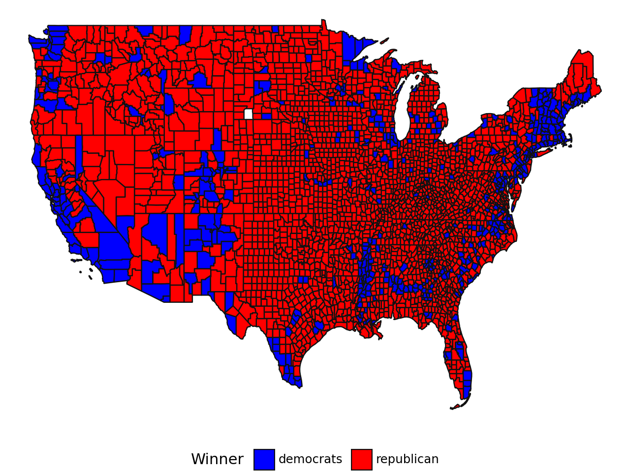
ImportantThe Territorial Trap
As mentioned in the chapter on mapping, choropleth maps can give a misleading impression that the Republican Party won by a large margin in 2020 because this type of graphic representation gives more importance to large areas rather than dense areas. This explains why this type of map has been used as justification for contesting the election results.
There are alternative representations better suited to such phenomena where density is significant. One such representation is proportional circles (see Insee (2018), “The Territorial Trap in Cartography”). Proportional circles allow the eye to focus on denser areas rather than large open spaces. With this representation, it becomes clear that the Democratic vote is in the majority, which was obscured by the flat color fill.
The GIF “Land does not vote, people do”, which gained popularity in 2020, offers another visualization approach. The original map was created with JavaScript. However, with Python, we have several tools to replicate this map at a low cost using one of the JavaScript overlays discussed in the visualization section.
Code pour reproduire cette carte interactive
import numpy as np
import pandas as pd
import geopandas as gpd
import plotly
import plotly.graph_objects as go


centroids = votes.copy()
centroids.geometry = centroids.centroid
centroids['size'] = centroids['CENSUS_2020_POP'] / 10000  # to get reasonable plotable number

color_dict = {"republican": '#FF0000', 'democrats': '#0000FF'}
centroids["winner"] =  np.where(centroids['votes_gop'] > centroids['votes_dem'], 'republican', 'democrats')


centroids['lon'] = centroids['geometry'].x
centroids['lat'] = centroids['geometry'].y
centroids = pd.DataFrame(
  centroids.loc[
    : ,
    ["county_name",'lon','lat','winner', 'CENSUS_2020_POP',"state_name"]
  ]
)
groups = centroids.groupby('winner')

df = centroids.copy()

df['color'] = df['winner'].replace(color_dict)
df['size'] = df['CENSUS_2020_POP']/6000
df['text'] = df['CENSUS_2020_POP'].astype(int).apply(lambda x: '<br>Population: {:,} people'.format(x))
df['hover'] = df['county_name'].astype(str) +  df['state_name'].apply(lambda x: ' ({}) '.format(x)) + df['text']

fig_plotly = go.Figure(
  data=go.Scattergeo(
  locationmode = 'USA-states',
  lon=df["lon"], lat=df["lat"],
  text = df["hover"],
  mode = 'markers',
  marker_color = df["color"],
  marker_size = df['size'],
  hoverinfo="text"
  )
)

fig_plotly.update_traces(
  marker = {'opacity': 0.5, 'line_color': 'rgb(40,40,40)', 'line_width': 0.5, 'sizemode': 'area'}
)

fig_plotly.update_layout(
  title_text = "Reproduction of the \"Acres don't vote, people do\" map <br>(Click legend to toggle traces)",
  showlegend = True,
  geo = {"scope": 'usa', "landcolor": 'rgb(217, 217, 217)'}
)

fig_plotly.show()
/tmp/ipykernel_10523/1328083585.py:9: UserWarning: Geometry is in a geographic CRS. Results from 'centroid' are likely incorrect. Use 'GeoSeries.to_crs()' to re-project geometries to a projected CRS before this operation.
2 General Approach
In this chapter, we will focus on data preparation to be done before modeling work. This step is essential to ensure consistency between the data and modeling assumptions and to produce scientifically valid analyses.
The general approach we will adopt in this chapter, which will be refined in subsequent chapters, is as follows:
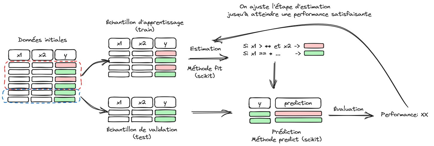
Figure 2.1 illustrates the structure of a machine learning problem.
First, the available dataset is split into two parts: training sample and validation sample. The former is used to train a model, and its prediction quality is evaluated on the latter to limit overfitting bias. The next chapter will delve deeper into model evaluation. At this stage of our progress, we will focus in this chapter on data issues.
The Scikit library is particularly convenient because it offers many machine learning algorithms with a few unified entry points, especially the fit and predict methods. However, the unification extends beyond algorithm training. All data preparation steps integrated into Scikit offer these same entry points. In other words, data preparations are built like parameter estimations that can be reapplied to another dataset. For example, this data preparation might be a mean and variance estimation for normalizing variables. The mean and variance are calculated on the training sample, and the same values can be reapplied to another dataset to normalize it in the same way.
3 Exploring data structure
The first necessary step before diving into modeling is to determine which variables to include in the model.
Pandas functionalities are sufficient at this stage for exploring simple structures.
However, when dealing with a dataset with numerous explanatory variables (features in machine learning, covariates in econometrics), it is often wise to start with a variable selection step, which we will cover later in the dedicated section.
Before selecting the best set of explanatory variables, we will start with a small and arbitrary selection. The first task is to represent the relationships within the data, particularly the relationship between explanatory variables and the dependent variable (the Republican Party’s score), as well as relationships among explanatory variables.
For the next exercise, to illustrate the principle of visual inspection of correlations, we’ll keep only a limited number of variables, chosen somewhat arbitrarily.
df2 = votes.set_index("GEOID").loc[
    : ,
    [
        "winner", "votes_gop",
        'Unemployment_rate_2019', 'Median_Household_Income_2021',
        'Percent of adults with less than a high school diploma, 2018-22',
        "Percent of adults with a bachelor's degree or higher, 2018-22"
    ]
]
df2 = df2.dropna()
TipExercise 2 (Optional): Examining Correlations Between Variables
This exercise is OPTIONAL
Use a graph to represent the correlation matrix. You can use the seaborn package and its heatmap function.
The correlation matrix can be constructed in various ways, depending on the framework you choose (see the chapter on visualization). The example below was produced using seaborn, which is well-suited for quick visualizations. However, considerable refinement would be needed to make the graphic suitable for publication.
Code to produce correlation matrix with seaborn
import numpy as np
import matplotlib.pyplot as plt
import seaborn as sns

column_labels = {
    'votes_gop': 'GOP votes',
    'Unemployment_rate_2019': 'Unemployment\n(2019)',
    'Median_Household_Income_2021': 'Median Income\n(2021)',
    'Percent of adults with less than a high school diploma, 2018-22': 'Less than HS diploma\n(2018–22)',
    'Percent of adults with a bachelor\'s degree or higher, 2018-22': 'Bachelor\'s degree or\nhigher (2018–22)'
}

corr = (
    df2.drop("winner", axis = 1)
    .rename(columns=column_labels)
    .corr()
)

mask = np.zeros_like(corr, dtype=bool)
mask[np.triu_indices_from(mask)] = True

# Set up the matplotlib figure
fig = plt.figure()

# Generate a custom diverging colormap
cmap = sns.diverging_palette(220, 10, as_cmap=True)

# Draw the heatmap with the mask and correct aspect ratio
g = sns.heatmap(
    corr,
    mask=mask,     # Mask upper triangular matrix
    cmap=cmap,
    annot=True,
    vmax=.3,
    vmin=-.3,
    center=0,      # The center value of the legend. With divergent cmap, where white is
    square=True,
    linewidths=.5,
    cbar_kws={"shrink": .5}
)

g
plt.xticks(rotation=30, ha='right')
plt.yticks(rotation=0)
plt.show()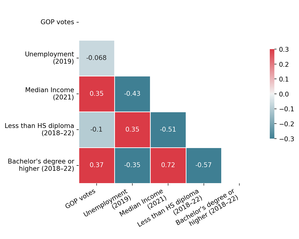
A similar but slightly cleaner figure can be produced using plotnine, the Python equivalent of the ggplot2 library in R (for more details, see the chapter on visualization). Since there is less online inspiration for plotnine - which is newer than matplotlib or seaborn - and fewer examples available compared to the rich ecosystem around R, the full code is provided below1.
Code to produce correlation matrix with plotnine
corr = (
    df2.drop("winner", axis = 1)
    .rename(columns=column_labels)
    .corr()
)

# 2. Transformation en format long
corr_long = corr.reset_index().melt(id_vars='index')
corr_long.columns = ['var1', 'var2', 'corr']

# 3. Supprimer la diagonale supérieure
corr_long['mask'] = corr_long.apply(lambda row: sorted([row['var1'], row['var2']]), axis=1)
corr_long['keep'] = corr_long['mask'].duplicated(keep='first')
corr_long = corr_long[~corr_long['keep']].drop(columns=['mask', 'keep'])

# 4. Ordre cohérent
var_order = corr.columns.tolist()
corr_long['var1'] = pd.Categorical(corr_long['var1'], categories=var_order, ordered=True)
corr_long['var2'] = pd.Categorical(corr_long['var2'], categories=var_order[::-1], ordered=True)

# 5. Groupe pour texte contrasté
corr_long['p_group'] = np.where(corr_long['corr'].abs() > 0.2, 'white', 'black')

# 5. Création du plot
p = (
    ggplot(corr_long, aes(x='var1', y='var2', fill='corr'))
    + geom_tile(width=0.95, height=0.95)
    + geom_text(aes(label='round(corr, 2)', color='p_group'), size=9, show_legend=False)
    + scale_fill_gradient2(low='blue', mid='white', high='red', midpoint=0, limits=(-1, 1))
    + scale_color_manual(values={'white': 'white', 'black': 'black'})
    + coord_fixed()
    + labs(x = "", y = "")
    + theme(
        axis_text_x=element_text(rotation=45, ha='right'),
        figure_size=(8, 6),
        panel_background=element_rect(fill='white'),
        legend_position = "none"
    )
)

p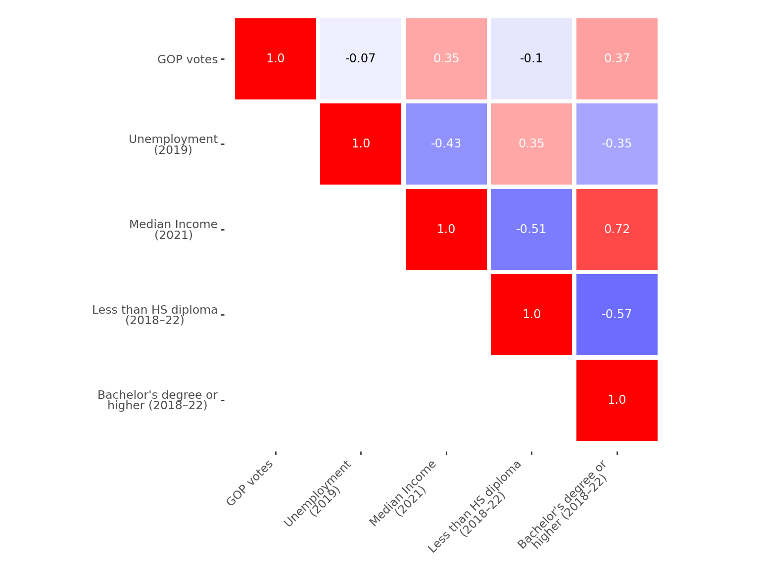
Last but not least, you can also build this correlation matrix with Plotly, even if it’s not the most practical ecosystem.
Code to produce correlation matrix with plotly
import plotly.express as px
import pandas as pd
import numpy as np

# Compute correlation matrix
corr = (
    df2.drop("winner", axis=1)
    .round(2)
    .rename(columns=column_labels)
    .corr()
)

# Mask upper triangle
mask = np.triu(np.ones_like(corr, dtype=bool))
corr_masked = corr.mask(mask)

# Plot heatmap
fig = px.imshow(
    corr_masked.values,
    x=corr.columns,
    y=corr.columns,
    color_continuous_scale='RdBu_r',  # <- reversed color scale
    zmin=-1,
    zmax=1,
    text_auto=".2f"
)

# Customize hover
fig.update_traces(
    hovertemplate="Var 1: %{y}<br>Var 2: %{x}<br>Corr: %{z:.2f}<extra></extra>"
)

# Layout tweaks
fig.update_layout(
    coloraxis_showscale=False,
    xaxis=dict(showticklabels=False, title=None, ticks=''),  # remove axis title and ticks
    yaxis=dict(showticklabels=True, title=None, ticks=''),
    plot_bgcolor="rgba(0,0,0,0)",
    margin=dict(t=10, b=10, l=10, r=10),  # <-- shrink ALL margins
    width=600,
    height=600
)

fig.show()As expected, the strongest correlations (in absolute value) are between income and education level. Income is also positively correlated with the Republican vote share. However, these results are purely descriptive and do not account for potential confounding factors. To explore these relationships more rigorously, we’ll need to introduce a modeling approach that can control for the interplay between variables.
4 Transforming data
Differences in scale or distribution between variables can diverge from the underlying assumptions in models.
For example, in linear regression, categorical variables are not treated the same way as variables with values in \(\mathbb{R}\). A discrete variable (taking a finite number of values) must be transformed into a sequence of 0/1 variables (dummies) relative to a reference category to meet the assumptions of linear regression. This type of transformation is known as one-hot encoding, which we will revisit. It is one of many transformations available in Scikit to align a dataset with mathematical assumptions.
All these data preparation tasks fall under preprocessing or feature engineering. One advantage of using Scikit is that preprocessing tasks can be considered learning tasks. Preprocessing involves learning parameters from a data structure (e.g., estimating means and variances to subtract from each observation), and these parameters can then be applied to observations not used to calculate them. In other words, this data preparation fits seamlessly into the pipeline shown in Figure 2.1.
4.1 Continuous Variable Preprocessing
We will cover two very common preprocessing steps for continuous variables:
Standardization transforms data so that the empirical distribution follows a \(\mathcal{N}(0,1)\) distribution.
Normalization transforms data to achieve a unit norm (\(\mathcal{l}_1\) or \(\mathcal{l}_2\)). In other words, with the appropriate norm, the sum of elements equals 1.
There are other options, such as MinMaxScaler to rescale variables according to observed minimum and maximum bounds. The choice of method depends on the algorithms chosen later: the assumptions of k-nearest neighbors (knn) differ from those of a random forest. For this reason, complete pipelines are usually defined, integrating both preprocessing and learning, which will be discussed in upcoming chapters.
CautionCaution
For statisticians,
the term normalization in Scikit terminology can have a counterintuitive meaning.
One might expect normalization to transform a variable so that \(X \sim \mathcal{N}(0,1)\).
In Scikit, this is actually standardization.
4.1.1 Standardization
Standardization involves transforming data so that the empirical distribution follows a \(\mathcal{N}(0,1)\) distribution. For optimal performance, most machine learning models often require data to follow this distribution. Even when it’s not essential, as with logistic regressions, it can speed up the convergence rate of algorithms.
TipExercise 3: Standardization
- Standardize the
Median_Household_Income_2021variable (do not overwrite the values!) and examine the histogram before and after normalization. This transformation should be applied to the entire column; the next questions will address sample splitting and extrapolation.
Note: This should yield a distribution centered at zero, and we could verify that the empirical variance is indeed 1. We could also check that this is true when transforming multiple columns at once.
- Create
scaler, aTransformerbuilt on the first 1000 rows of yourdf2DataFrame, excluding the target variablewinner. Check the mean and standard deviation of each column for these same observations.
Note: The parameters used for subsequent standardization are stored in the .mean_ and .scale_ attributes.
These attributes can be seen as parameters trained on a specific dataset that can be reused on another, as long as the dimensions match.
- Apply
scalerto the remaining rows of the DataFrame and compare the distributions obtained for theMedian_Household_Income_2021variable.
Note: Once applied to another DataFrame, you may notice that the distribution is not exactly standardized in the DataFrame on which the parameters were not estimated. This is normal; the initial sample was not random, so the means and variances of this sample do not necessarily match those of the complete sample.
Before standardization, our variable has this distribution:
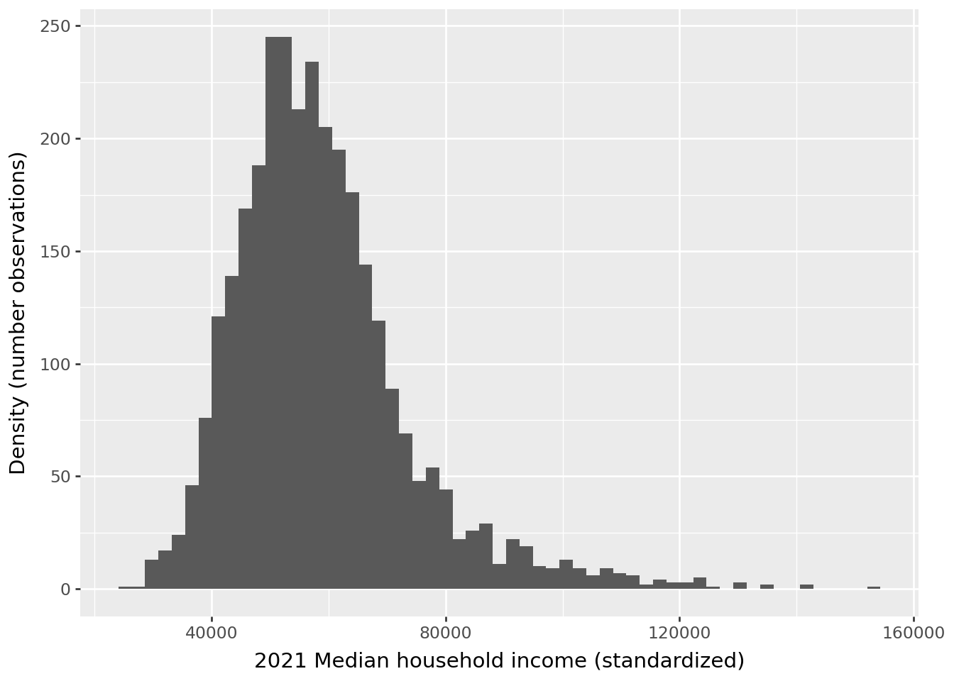
After standardization, the scale of the variable has changed.
/home/runner/work/python-datascientist/python-datascientist/.venv/lib/python3.13/site-packages/plotnine/stats/stat_bin.py:112: PlotnineWarning: 'stat_bin()' using 'bins = 57'. Pick better value with 'binwidth'.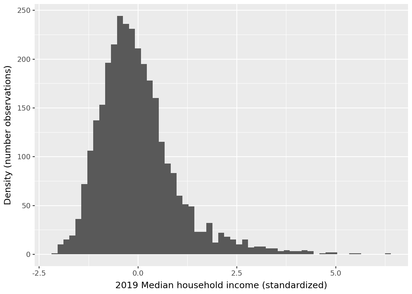
We indeed obtain a mean equal to 0 and a variance equal to 1, within numerical approximations:
| Statistique | Valeur | |
|---|---|---|
| 0 | Mean | 0.000000 |
| 1 | Variance | 1.000323 |
For question 2, if we attempt to present the obtained statistics in a readable table, we get
| Variable | Mean before Scaling | Std before Scaling | Mean after Scaling | Std after Scaling |
|---|---|---|---|---|
| votes_gop | ||||
| Unemployment_rate_2019 | ||||
| Median_Household_Income_2021 | ||||
| Percent of adults with less than a high school diploma, 2018-22 | ||||
| Percent of adults with a bachelor's degree or higher, 2018-22 | ||||
| y_standard |
It is very clear from this table that the standardization worked well.
Now, if we create a formal transformer for our variables (question 3)
StandardScaler()In a Jupyter environment, please rerun this cell to show the HTML representation or trust the notebook.
On GitHub, the HTML representation is unable to render, please try loading this page with nbviewer.org.
Parameters
We can extrapolate our standardizer to a larger dataset. If we look at the distribution obtained on the first 1000 rows (question 3), we find a scale consistent with a \(\mathcal{N(0,1)}\) distribution for the unemployment variable:
However, we see that this distribution does not correspond to the one that would truly normalize the rest of the data.
This is an illustration of a classic problem in machine learning, called data drift, which occurs when we attempt to extrapolate to data whose distribution no longer corresponds to that of the training data. This situation typically arises when an algorithm has been trained on a biased sample of the population or when we have non-stationary time series data. It is, therefore, essential to carefully consider the construction of the training sample and the potential for extrapolation to a broader population: the external validity of the model—whether data preparation or learning algorithm—can be null if this step was rushed.
ImportantData Drift
Data drift refers to a shift in data distribution over time, leading to a degradation in the performance of a machine learning model that, by design, was trained on past data.
This phenomenon can occur due to changes in the target population, shifts in data characteristics, or external factors.
Detecting data drift is crucial to adjust or retrain the model, ensuring its relevance and accuracy. Detection techniques include statistical tests and monitoring specific metrics.
4.1.2 Normalization
Normalization is the process of transforming data to achieve a unit norm (\(\mathcal{l}_1\) or \(\mathcal{l}_2\)).
In other words, with the appropriate norm, the sum of elements equals 1.
By default, Scikit uses an \(\mathcal{l}_2\) norm.
This transformation is especially useful in text classification or clustering.
This is also an opportunity to explore how to split data into multiple samples using the train_test_split function in Scikit. We will create a 70% sample of the data to estimate normalization parameters (training phase) and extrapolate to the remaining 30%. This split is fairly standard but, of course, adaptable depending on the project. The advantage of using train_test_split instead of manually sampling with Pandas’ sample method is that Scikit’s function allows for much more control over sampling, particularly if stratification is desired, while being reliable. Doing this manually can be tedious and risky, as it is potentially complex to implement without errors.
TipExercise 4: Normalization
- Using the documentation for the
train_test_splitfunction inScikit, create two samples (70% and 30% of the data, respectively). - Normalize the
Median_Household_Income_2021variable (do not overwrite the values!) and examine the histogram before and after normalization. - Verify that the \(\mathcal{l}_2\) norm is indeed equal to 1 (using the
np.linalg.normfunction with theaxis=1argument) for the first 10 observations in the training set and then for the other observations.
/home/runner/work/python-datascientist/python-datascientist/.venv/lib/python3.13/site-packages/plotnine/stats/stat_bin.py:112: PlotnineWarning: 'stat_bin()' using 'bins = 51'. Pick better value with 'binwidth'.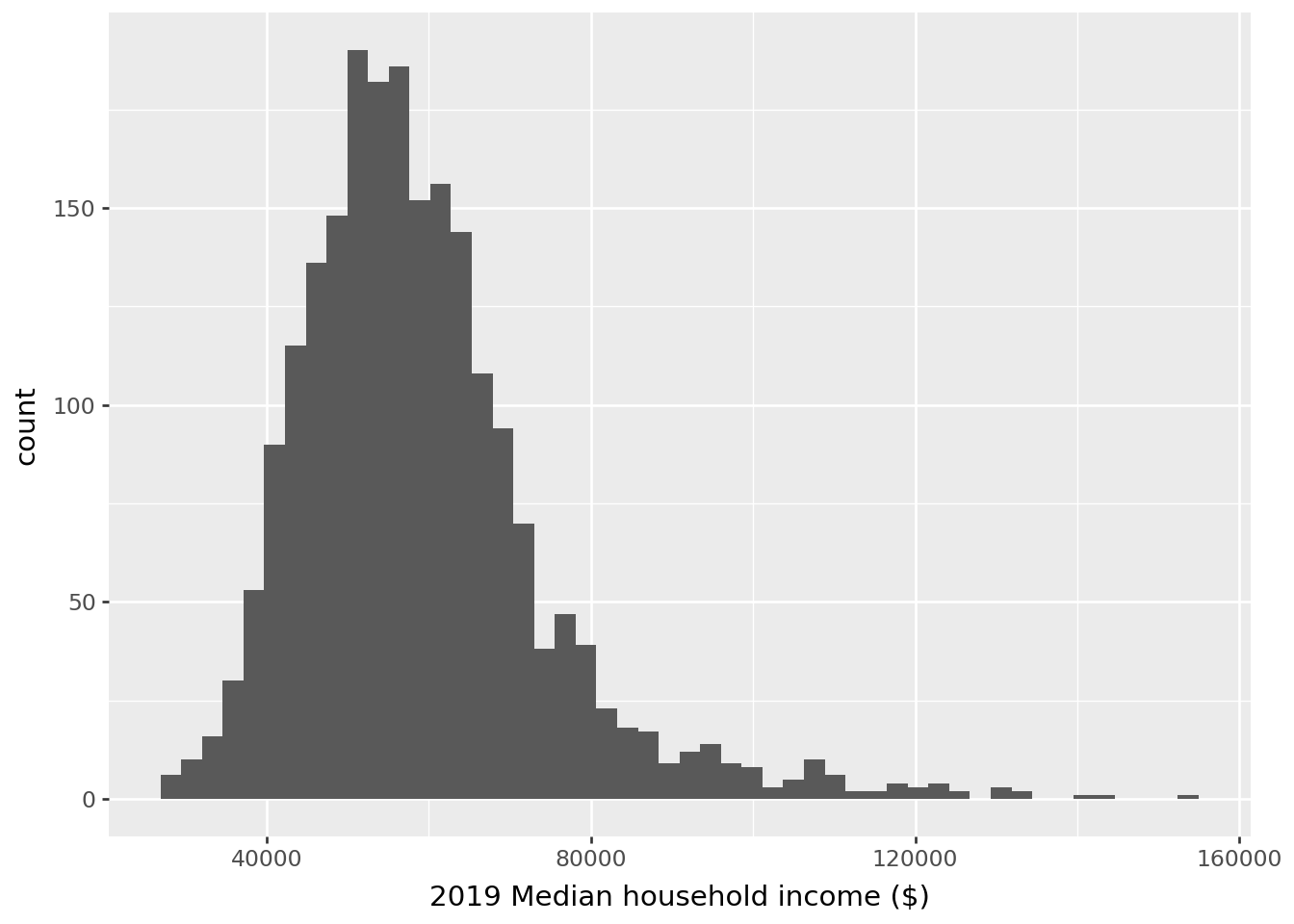
/home/runner/work/python-datascientist/python-datascientist/.venv/lib/python3.13/site-packages/plotnine/stats/stat_bin.py:112: PlotnineWarning: 'stat_bin()' using 'bins = 113'. Pick better value with 'binwidth'.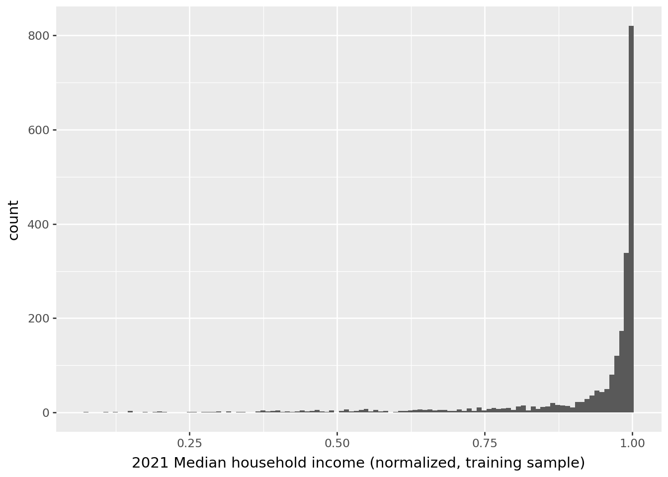
/home/runner/work/python-datascientist/python-datascientist/.venv/lib/python3.13/site-packages/plotnine/stats/stat_bin.py:112: PlotnineWarning: 'stat_bin()' using 'bins = 92'. Pick better value with 'binwidth'.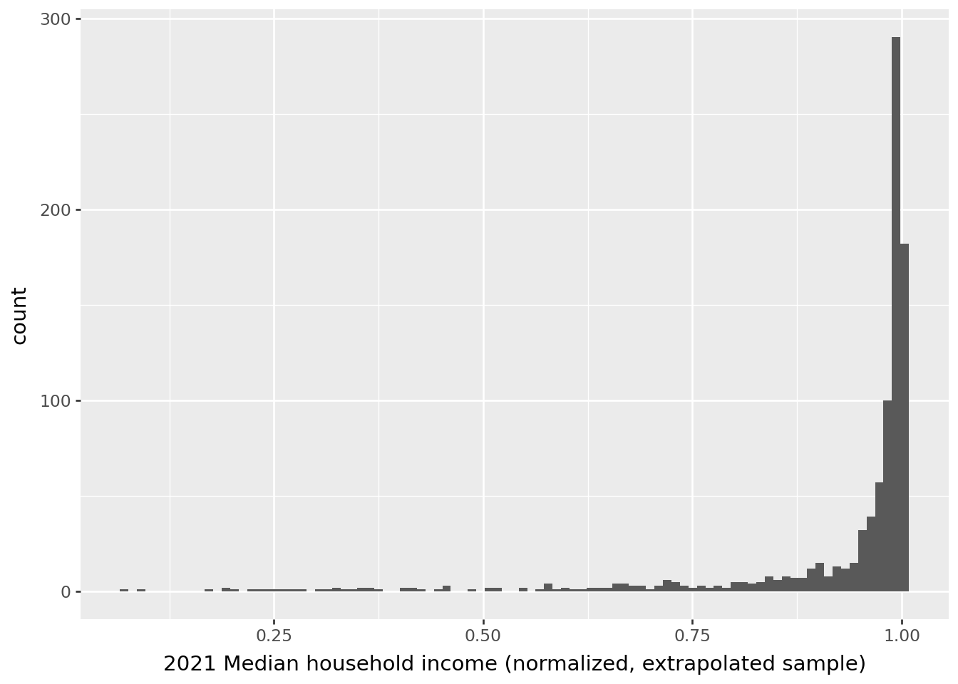
Finally, if we compute the norm, we obtain the expected result on both the train sample and the extrapolated sample.
| X_train_norm2 | X_test_norm2 | |
|---|---|---|
| 0 | 1.0 | 1.0 |
| 1 | 1.0 | 1.0 |
| 2 | 1.0 | 1.0 |
| 3 | 1.0 | 1.0 |
| 4 | 1.0 | 1.0 |
4.2 Encoding Categorical Values
Categorical data must be recoded into numeric values to be integrated into machine learning models.
This can be done in several ways with Scikit:
LabelEncoder: transforms a vector["a","b","c"]into a numeric vector[0,1,2]. This approach has the drawback of introducing an order to the categories, which is not always desirable.OrdinalEncoder: a generalized version ofLabelEncoderdesigned to apply to matrices (\(X\)), whileLabelEncoderapplies mainly to a vector (\(y\)).
For one-hot encoding, several methods are available:
pandas.get_dummiesperforms a dummy expansion. A vector of size n with K categories will be transformed into a matrix of size \(n \times K\), where each column represents a dummy variable for category k. There are \(K\) categories, resulting in multicollinearity. In linear regression with a constant, one category should be removed before estimation.OneHotEncoderis a generalized (and optimized) version of dummy expansion. This is the recommended method.
4.3 Imputation
Data often contains missing values, that is, observations in our DataFrame containing a NaN. These gaps can cause bugs or misinterpretations when moving to modeling.
One initial approach could be to remove all observations with a NaN in at least one column.
However, if our table contains many NaNs, or if these are spread across numerous columns,
we risk removing a significant number of rows, and, with that, losing important information, as missing values are rarely randomly distributed.
While this solution remains viable in many cases, a more robust approach called imputation exists. This method involves replacing missing values with a specified value. For example:
- Mean imputation: replacing all
NaNs in a column with the column’s average; - Median imputation on the same principle, or using the most frequent column value for categorical variables;
- Regression imputation: using other variables to interpolate an appropriate replacement value.
More complex methods are available, but in many cases, the above approaches can provide much more satisfactory results.
The Scikit package makes imputation very straightforward (documentation here).
4.4 Handling Outliers
Outliers are observations that significantly deviate from the general trend of other observations in a dataset. In other words, they are data points that stand out unusually from the overall data distribution. This may be due to data entry errors, respondents who incorrectly answered a survey, or simply extreme values that may bias a model too much.
For example, these could be 3 individuals measuring over 4 meters in height within a population or household incomes exceeding 10 million euros per month at a national level.
It is good practice to routinely examine the distribution of available variables to check if some values deviate too significantly from others. Sometimes these values will interest us, for instance, if we are focusing solely on very high incomes (top 0.1%) in France. However, often these values will be more of a hindrance, especially if they don’t make sense in the real world.
If we find that the presence of these extreme values or outliers in our dataset is more problematic than helpful, it is reasonable to simply remove them. Most of the time, we set a percentage of data to remove, such as 0.1%, 1%, or 5%, then remove the corresponding extreme values in both tails of the distribution.
Several packages can perform these operations, which can become complex if we examine outliers across multiple variables.
The IsolationForest() function in the sklearn.ensemble package is particularly noteworthy.
4.5 Application exercise
CautionBe careful with new categories!
Transformers create a mapping between text categories and numeric values. This assumes that the data used to build this mapping includes all possible values for the text categories.
However, if new categories appear, the classifier will not know how to transform these into numeric values, which will cause an error in Scikit. This technical error makes sense, as it would require updating not only the mapping but also the estimation of underlying parameters.
TipExercise 5: Encoding Categorical Variables
Create
dfthat retains only thestate_nameandcounty_namevariables invotes.Apply a
LabelEncodertostate_nameNote: The label encoding result is relatively intuitive, especially when related to the initial vector.Observe the dummy expansion of
state_nameApply an
OrdinalEncodertodf.loc[:, ['state_name', 'county_name']]Note: The ordinal encoding result is consistent with the label encodingApply a
OneHotEncodertodf.loc[:, ['state_name', 'county_name']]
Note: scikit optimizes the object required to store the result of a transformation model. For example, the One Hot encoding result is a very large object. In this case, scikit uses a Sparse matrix.
If we examine the labels and their numeric transpositions via LabelEncoder
array([[23, 'Missouri'],
       [25, 'Nebraska'],
       [30, 'New York'],
       ...,
       [41, 'Texas'],
       [41, 'Texas'],
[41, 'Texas']], shape=(3108, 2), dtype=object)| Alabama | Arizona | Arkansas | California | Colorado | Connecticut | Delaware | District of Columbia | Florida | Georgia | ... | South Dakota | Tennessee | Texas | Utah | Vermont | Virginia | Washington | West Virginia | Wisconsin | Wyoming | |
|---|---|---|---|---|---|---|---|---|---|---|---|---|---|---|---|---|---|---|---|---|---|
| 0 | False | False | False | False | False | False | False | False | False | False | ... | False | False | False | False | False | False | False | False | False | False |
| 1 | False | False | False | False | False | False | False | False | False | False | ... | False | False | False | False | False | False | False | False | False | False |
| 2 | False | False | False | False | False | False | False | False | False | False | ... | False | False | False | False | False | False | False | False | False | False |
| 3 | False | False | False | False | False | False | False | False | False | False | ... | False | False | False | False | False | False | False | False | False | False |
| 4 | False | False | False | False | False | False | False | False | False | False | ... | False | True | False | False | False | False | False | False | False | False |
| ... | ... | ... | ... | ... | ... | ... | ... | ... | ... | ... | ... | ... | ... | ... | ... | ... | ... | ... | ... | ... | ... |
| 3103 | False | False | False | False | False | False | False | False | False | False | ... | False | False | False | False | False | False | False | False | False | False |
| 3104 | False | False | False | False | False | False | False | False | False | False | ... | False | False | False | False | False | False | False | False | False | False |
| 3105 | False | False | False | False | False | False | False | False | False | False | ... | False | False | True | False | False | False | False | False | False | False |
| 3106 | False | False | False | False | False | False | False | False | False | False | ... | False | False | True | False | False | False | False | False | False | False |
| 3107 | False | False | False | False | False | False | False | False | False | False | ... | False | False | True | False | False | False | False | False | False | False |
3108 rows × 49 columns
If we examine the OrdinalEncoder:
array([23., 25., 30., ..., 41., 41., 41.], shape=(3108,))<Compressed Sparse Row sparse matrix of dtype 'float64'
with 6216 stored elements and shape (3108, 1892)>Reference
Insee. 2018. “Guide de Sémiologie Cartographique.”
Informations additionnelles
NotePython environment
This site was built automatically through a Github action using the Quarto
The environment used to obtain the results is reproducible via uv. The pyproject.toml file used to build this environment is available on the linogaliana/python-datascientist repository
pyproject.toml
[project]
name = "python-datascientist"
version = "0.1.0"
description = "Source code for Lino Galiana's Python for data science course"
readme = "README.md"
requires-python = ">=3.13,<3.14"
dependencies = [
    "altair>=6.0.0",
    "cartiflette",
    "contextily==1.6.2",
    "duckdb>=0.10.1",
    "folium>=0.19.6",
    "gdal==3.11.4",
    "graphviz==0.20.3",
    "great-tables>=0.12.0",
    "gt-extras>=0.0.8",
    "ipykernel>=6.29.5",
    "jupyter>=1.1.1",
    "jupyter-cache>=1.0.0",
    "kaleido>=0.2.1",
    "langchain-community>=0.3.27",
    "loguru==0.7.3",
    "markdown>=3.8",
    "nbclient>=0.10.0",
    "nbformat>=5.10.4",
    "nltk>=3.9.1",
    "pandas>=2.3.3",
    "pip>=25.1.1",
    "plotly>=6.1.2",
    "plotnine>=0.15",
    "polars>=1.8.2",
    "pyarrow>=17.0.0",
    "pynsee>=0.1.8",
    "python-dotenv>=1.0.1",
    "python-frontmatter>=1.1.0",
    "pywaffle>=1.1.1",
    "requests>=2.32.3",
    "scikit-image>=0.24.0",
    "scikit-learn>=1.8.0",
    "scipy>=1.13.0",
    "seaborn>=0.13.2",
    "selenium<4.39.0",
    "spacy>=3.8.4",
    "webdriver-manager>=4.0.2",
    "wordcloud==1.9.3",
]

[tool.uv.sources]
cartiflette = { git = "https://github.com/inseefrlab/cartiflette" }
gdal = [
  { index = "gdal-wheels", marker = "sys_platform == 'linux'" },
  { index = "geospatial_wheels", marker = "sys_platform == 'win32'" },
]

[[tool.uv.index]]
name = "geospatial_wheels"
url = "https://nathanjmcdougall.github.io/geospatial-wheels-index/"
explicit = true

[[tool.uv.index]]
name = "gdal-wheels"
url = "https://gitlab.com/api/v4/projects/61637378/packages/pypi/simple"
explicit = true

[dependency-groups]
dev = [
    "nb-clean>=4.0.1",
]
To use exactly the same environment (version of Python and packages), please refer to the documentation for uv.
NoteFile history
| SHA | Date | Author | Description |
|---|---|---|---|
| cf502001 | 2025-12-22 13:38:37 | Lino Galiana | Update de l’environnement (et retrait de yellowbricks au passage) (#665) |
| c216d383 | 2025-11-25 10:43:19 | lgaliana | Corrige typo loc pandas |
| d56f6e9e | 2025-11-25 08:30:59 | lgaliana | Un petit coup de neuf sur les consignes et corrections pandas related |
| c3d51646 | 2025-08-12 17:28:51 | Lino Galiana | Ajoute un résumé au début de chaque chapitre (première partie) (#634) |
| 8fe46396 | 2025-08-12 14:02:32 | lgaliana | Figures de la partie modélisation |
| 99ab48b0 | 2025-07-25 18:50:15 | Lino Galiana | Utilisation des callout classiques pour les box notes and co (#629) |
| 94648290 | 2025-07-22 18:57:48 | Lino Galiana | Fix boxes now that it is better supported by jupyter (#628) |
| 91431fa2 | 2025-06-09 17:08:00 | Lino Galiana | Improve homepage hero banner (#612) |
| 48dccf14 | 2025-01-14 21:45:34 | lgaliana | Fix bug in modeling section |
| 64c12dc5 | 2024-11-07 19:28:22 | lgaliana | English version |
| e945ff4a | 2024-11-07 18:02:05 | lgaliana | update |
| 1a8267a1 | 2024-11-07 17:11:44 | lgaliana | Finalize chapter and fix problem |
| 63b581f6 | 2024-11-07 10:48:51 | lgaliana | Normalisation |
| a2517095 | 2024-11-07 09:31:19 | lgaliana | Exemple |
| e0728909 | 2024-11-06 18:17:32 | lgaliana | Continue le cleaning |
| f3bbddce | 2024-11-06 16:48:47 | lgaliana | Commence revoir premier chapitre modélisation |
| c641de05 | 2024-08-22 11:37:13 | Lino Galiana | A series of fix for notebooks that were bugging (#545) |
| 1cdcd273 | 2024-08-08 07:19:23 | linogaliana | change url |
| 580cba77 | 2024-08-07 18:59:35 | Lino Galiana | Multilingual version as quarto profile (#533) |
| 06d003a1 | 2024-04-23 10:09:22 | Lino Galiana | Continue la restructuration des sous-parties (#492) |
| 005d89b8 | 2023-12-20 17:23:04 | Lino Galiana | Finalise l’affichage des statistiques Git (#478) |
| 3fba6124 | 2023-12-17 18:16:42 | Lino Galiana | Remove some badges from python (#476) |
| 417fb669 | 2023-12-04 18:49:21 | Lino Galiana | Corrections partie ML (#468) |
| 1f23de28 | 2023-12-01 17:25:36 | Lino Galiana | Stockage des images sur S3 (#466) |
| a06a2689 | 2023-11-23 18:23:28 | Antoine Palazzolo | 2ème relectures chapitres ML (#457) |
| b68369d4 | 2023-11-18 18:21:13 | Lino Galiana | Reprise du chapitre sur la classification (#455) |
| fd3c9557 | 2023-11-18 14:22:38 | Lino Galiana | Formattage des chapitres scikit (#453) |
| 889a71ba | 2023-11-10 11:40:51 | Antoine Palazzolo | Modification TP 3 (#443) |
| 9a4e2267 | 2023-08-28 17:11:52 | Lino Galiana | Action to check URL still exist (#399) |
| a8f90c2f | 2023-08-28 09:26:12 | Lino Galiana | Update featured paths (#396) |
| 80823022 | 2023-08-25 17:48:36 | Lino Galiana | Mise à jour des scripts de construction des notebooks (#395) |
| 3bdf3b06 | 2023-08-25 11:23:02 | Lino Galiana | Simplification de la structure 🤓 (#393) |
| 78ea2cbd | 2023-07-20 20:27:31 | Lino Galiana | Change titles levels (#381) |
| 29ff3f58 | 2023-07-07 14:17:53 | linogaliana | description everywhere |
| f21a24d3 | 2023-07-02 10:58:15 | Lino Galiana | Pipeline Quarto & Pages 🚀 (#365) |
| ebca985b | 2023-06-11 18:14:51 | Lino Galiana | Change handling precision (#361) |
| 129b0012 | 2022-12-26 20:36:01 | Lino Galiana | CSS for ipynb (#337) |
| f5f0f9c4 | 2022-11-02 19:19:07 | Lino Galiana | Relecture début partie modélisation KA (#318) |
| f10815b5 | 2022-08-25 16:00:03 | Lino Galiana | Notebooks should now look more beautiful (#260) |
| 494a85ae | 2022-08-05 14:49:56 | Lino Galiana | Images featured ✨ (#252) |
| d201e3cd | 2022-08-03 15:50:34 | Lino Galiana | Pimp la homepage ✨ (#249) |
| 640b9605 | 2022-06-10 15:42:04 | Lino Galiana | Finir de régler le problème plotly (#236) |
| 5698e303 | 2022-06-03 18:28:37 | Lino Galiana | Finalise widget (#232) |
| 7b9f27be | 2022-06-03 17:05:15 | Lino Galiana | Essaie régler les problèmes widgets JS (#231) |
| 12965bac | 2022-05-25 15:53:27 | Lino Galiana | :launch: Bascule vers quarto (#226) |
| 9c71d6e7 | 2022-03-08 10:34:26 | Lino Galiana | Plus d’éléments sur S3 (#218) |
| 8f99cd32 | 2021-12-08 15:26:28 | linogaliana | hide otuput |
| 9c5f718d | 2021-12-08 14:36:59 | linogaliana | format dico :sob: |
| 41c89864 | 2021-12-08 14:25:18 | linogaliana | correction erreur |
| 64747466 | 2021-12-08 14:08:06 | linogaliana | dict ici aussi |
| 8e73912d | 2021-12-08 12:32:17 | linogaliana | coquille plotly :sob: |
| 37042139 | 2021-12-08 11:57:51 | linogaliana | essaye avec un dict classique |
| 85565d5c | 2021-12-08 08:15:29 | linogaliana | reformat |
| 9ace7b92 | 2021-12-07 17:49:18 | linogaliana | évite la boucle crado |
| 3514e090 | 2021-12-07 16:05:28 | linogaliana | sépare et document |
| 63e67e67 | 2021-12-07 15:15:34 | Lino Galiana | Debug du plotly (temporaire) (#193) |
| 65cecdd8 | 2021-12-07 10:29:18 | Lino Galiana | Encore une erreur de nom de colonne (#192) |
| 81b7023a | 2021-12-07 09:27:35 | Lino Galiana | Mise à jour liste des colonnes (#191) |
| c3bf4d42 | 2021-12-06 19:43:26 | Lino Galiana | Finalise debug partie ML (#190) |
| d91a5eb1 | 2021-12-06 18:53:33 | Lino Galiana | La bonne branche c’est master |
| d86129c0 | 2021-12-06 18:02:32 | Lino Galiana | verbose |
| fb14d406 | 2021-12-06 17:00:52 | Lino Galiana | Modifie l’import du script (#187) |
| 37ecfa3c | 2021-12-06 14:48:05 | Lino Galiana | Essaye nom différent (#186) |
| 2c8fd0dd | 2021-12-06 13:06:36 | Lino Galiana | Problème d’exécution du script import data ML (#185) |
| 5d0a5e38 | 2021-12-04 07:41:43 | Lino Galiana | MAJ URL script recup data (#184) |
| 5c104904 | 2021-12-03 17:44:08 | Lino Galiana | Relec (antuki?) partie modelisation (#183) |
| 2a8809fb | 2021-10-27 12:05:34 | Lino Galiana | Simplification des hooks pour gagner en flexibilité et clarté (#166) |
| 2e4d5862 | 2021-09-02 12:03:39 | Lino Galiana | Simplify badges generation (#130) |
| 49e2826f | 2021-05-13 18:11:20 | Lino Galiana | Corrige quelques images n’apparaissant pas (#108) |
| 4cdb759c | 2021-05-12 10:37:23 | Lino Galiana | :sparkles: :star2: Nouveau thème hugo :snake: :fire: (#105) |
| 7f9f97bc | 2021-04-30 21:44:04 | Lino Galiana | 🐳 + 🐍 New workflow (docker 🐳) and new dataset for modelization (2020 🇺🇸 elections) (#99) |
| 347f50f3 | 2020-11-12 15:08:18 | Lino Galiana | Suite de la partie machine learning (#78) |
| 671f75a4 | 2020-10-21 15:15:24 | Lino Galiana | Introduction au Machine Learning (#72) |
Footnotes
This version was generated with the help of
ChatGPTin just a few seconds, sparing me the trouble of figuring out the ideal data structure to replicate the heatmap example from theplotninedocumentation.↩︎
Citation
BibTeX citation:
@book{galiana2025,
  author = {Galiana, Lino},
  title = {Python Pour La Data Science},
  date = {2025},
  url = {https://pythonds.linogaliana.fr/},
  doi = {10.5281/zenodo.8229676},
  langid = {en}
}
For attribution, please cite this work as:
Galiana, Lino. 2025. Python Pour La Data Science. https://doi.org/10.5281/zenodo.8229676.