# Sur colab
1!pip install pandas fiona shapely pyproj rtree geopandas- 1
- Ces librairies sont utiles pour l’analyse géospatiale (cf. chapitre dédié)

With the proliferation of geolocated data and the increasing use of data-driven decision-making, it has become crucial for data scientists to quickly create maps. This chapter, complementing the one on spatial data, offers exercises to explore the key principles of data visualization through cartography using Python.
Cartography is one of the oldest forms of graphical representation of information. Historically confined to military and administrative uses or navigation-related information synthesis, cartography has, at least since the 19th century, become one of the preferred ways to represent information. It was during this period that the color-shaded map, known as the choropleth map, began to emerge as a standard way to visualize geographic data.
According to Chen et al. (2008), the first representation of this type was proposed by Charles Dupin in 1826 Figure 1.1 to illustrate literacy levels across France. The rise of choropleth maps is closely linked to the organization of power through unitary political entities. For instance, world maps often use color shades to represent nations, while national maps use administrative divisions (regions, departments, municipalities, as well as states or Länder).
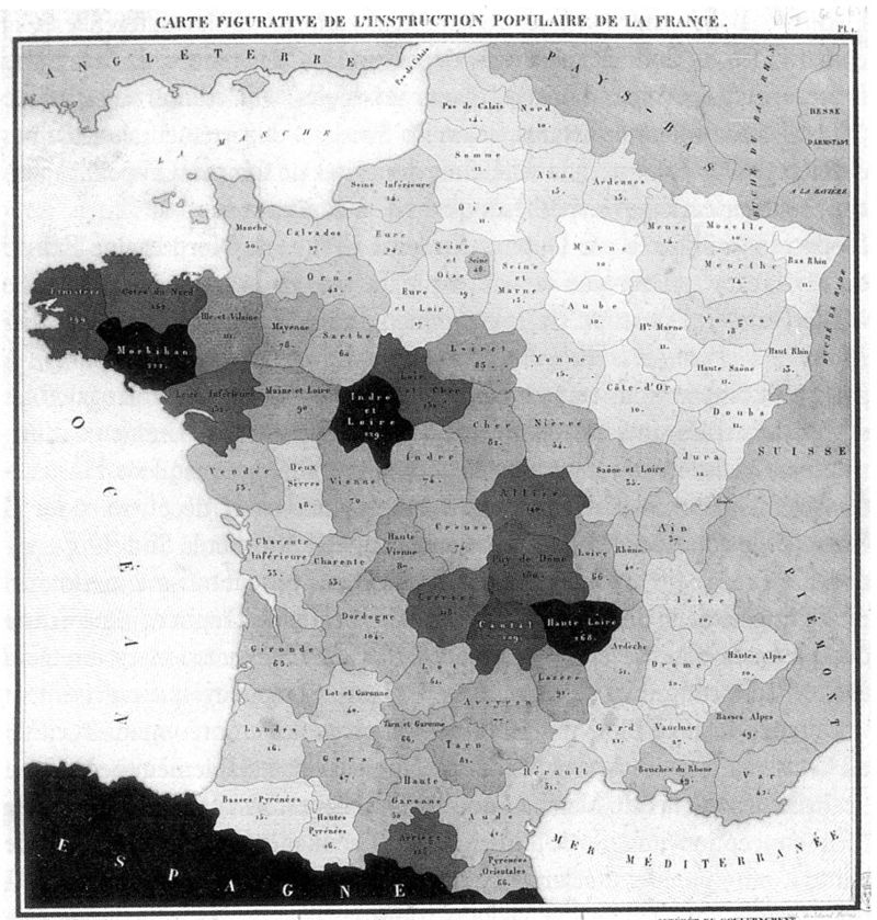
The emergence of choropleth maps during the 19th century marks an important shift in cartography, transitioning from military use to political application. No longer limited to depicting physical terrain, maps began to represent socioeconomic realities within well-defined administrative boundaries.
Creating high-quality maps requires time but also thoughtful decision-making. Like any graphical representation, it is essential to consider the message being conveyed and the most appropriate means of representation. Cartographic semiology, a scientific discipline focusing on the messages conveyed by maps, provides guidelines to prevent misleading representations—whether intentional or accidental.
Some of these principles are outlined in this cartographic semiology guide from Insee. They are also summarized in this guide.
This presentation by Nicolas Lambert, using numerous examples, explores key principles of cartographic dataviz.
This chapter will first introduce some basic functionalities of Geopandas for creating static maps. To provide context to the presented information, we will use official geographic boundaries produced by IGN. We will then explore maps with enhanced contextualization and multiple levels of information, illustrating the benefits of using interactive libraries based on JavaScript, such as Folium.
Throughout this chapter, we will use several datasets to illustrate different types of maps:
Before getting started, a few packages need to be installed:
# Sur colab
1!pip install pandas fiona shapely pyproj rtree geopandasWe will primarily need Pandas and GeoPandas for this chapter.
import pandas as pd
import geopandas as gpdWe will use cartiflette, which simplifies the retrieval of administrative basemaps from IGN. This package is an interministerial project designed to provide a simple Python interface for obtaining official IGN boundaries.
First, we will retrieve the departmental boundaries:
from cartiflette import carti_download
departements = carti_download(
values="France",
crs=4326,
borders="DEPARTEMENT",
vectorfile_format="geojson",
filter_by="FRANCE_ENTIERE_DROM_RAPPROCHES",
source="EXPRESS-COG-CARTO-TERRITOIRE",
year=2022,
)These data bring the DROM closer to mainland France, as explained in one of the cartiflette tutorials and as Exercise 1 will allow us to verify.
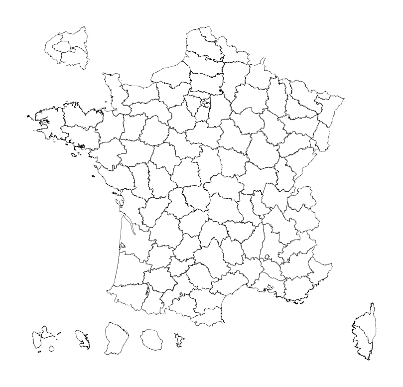
Exercise 1 aims to ensure that we have correctly retrieved the desired boundaries by simply visualizing them. This should be the first reflex of any geodata scientist.
plot method on the departements dataset to check the spatial extent. What projection do the displayed coordinates suggest? Verify using the crs method.matplotlib options, create a map with black boundaries, a white background, and no axes.The map of the departments, without modifying any options, looks like this:
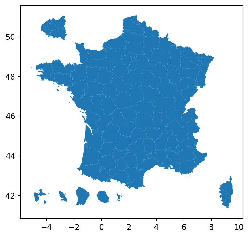
The displayed coordinates suggest WGS84, which can be verified using the crs method:
<Geographic 2D CRS: EPSG:4326>
Name: WGS 84
Axis Info [ellipsoidal]:
- Lat[north]: Geodetic latitude (degree)
- Lon[east]: Geodetic longitude (degree)
Area of Use:
- name: World.
- bounds: (-180.0, -90.0, 180.0, 90.0)
Datum: World Geodetic System 1984 ensemble
- Ellipsoid: WGS 84
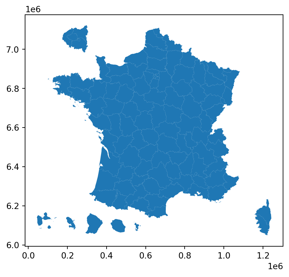
- Prime Meridian: GreenwichIf we convert to Lambert 93 (the official system for mainland France), we obtain a different extent, which is supposed to be more accurate for the mainland (but not for the relocated DROM, since, for example, French Guiana is actually much larger).
And of course, we can easily reproduce the failed maps from the chapter on GeoPandas, for example, if we apply a transformation designed for North America:
departements.to_crs(5070).plot()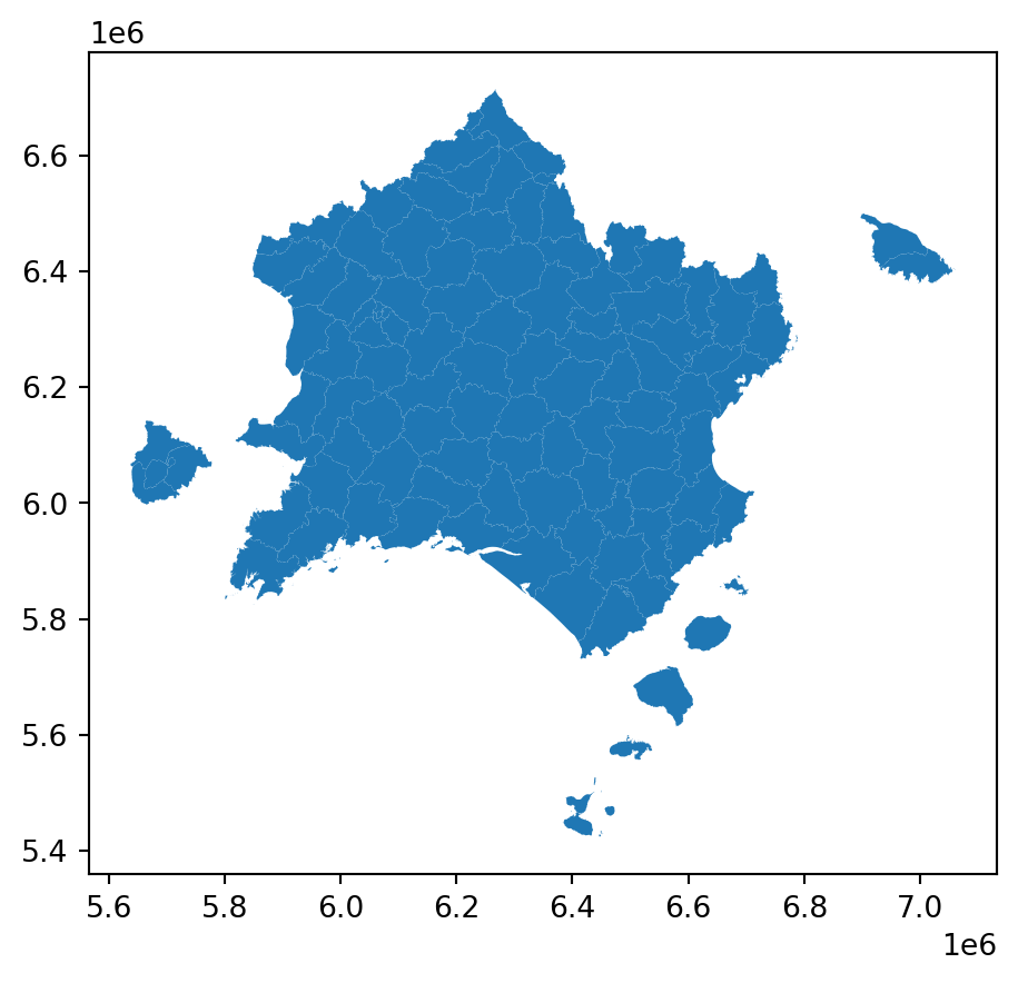
If we create a slightly more aesthetically pleasing map, we get:
And the same for Finistère:
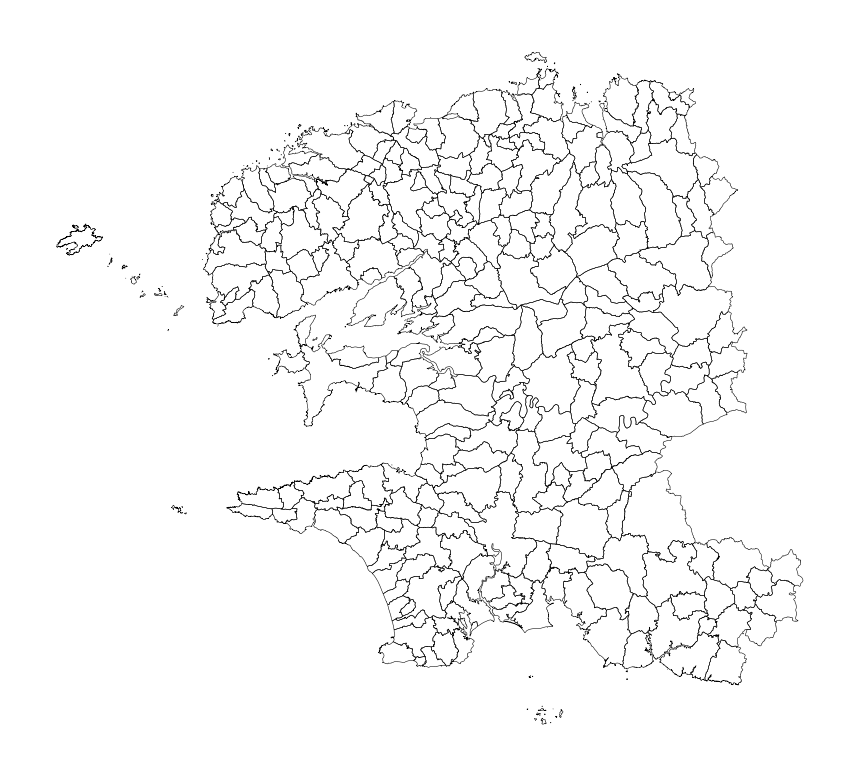
These maps are simple, yet they already rely on implicit knowledge. They require familiarity with the territory. When we start coloring certain departments, recognizing which ones have extreme values will require a good understanding of French geography. Likewise, while it may seem obvious, nothing in our map of Finistère explicitly states that the department is bordered by the ocean. A French reader would see this as self-evident, but a foreign reader, who may not be familiar with the details of our geography, would not necessarily know this.
To address this, we can use interactive maps that allow:
For this, we will retain only the data corresponding to an actual spatial extent, excluding our zoom on Île-de-France and the DROM.
We successfully obtain the hexagon:
departements_hexagone.plot()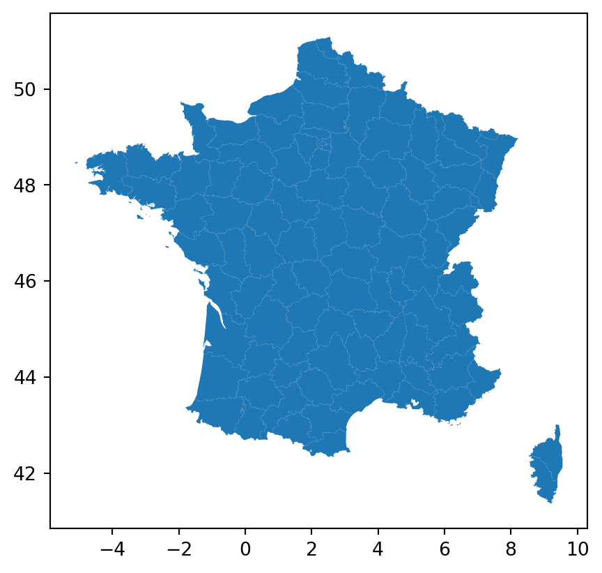
For the next exercise, we will need a few additional variables. First, the geometric center of France, which will help us position the center of our map.
minx, miny, maxx, maxy = departements_hexagone.total_bounds
center = [(miny + maxy) / 2, (minx + maxx) / 2]We will also need a dictionary to provide Folium with information about our map parameters.
style_function = lambda x: {
1 'fillColor': 'white',
'color': 'black',
'weight': 1.5,
'fillOpacity': 0.0
}fillOpacity parameter set to 0%.
style_function is an anonymous function that will be used in the exercise.
Information that appears when hovering over an element is called a tooltip in web development terminology.
import folium
tooltip = folium.GeoJsonTooltip(
fields=['LIBELLE_DEPARTEMENT', 'INSEE_DEP', 'POPULATION'],
aliases=['Département:', 'Numéro:', 'Population:'],
localize=True
)For the next exercise, the GeoDataFrame must be in the Mercator projection. Folium requires data in this projection because it relies on navigation basemaps, which are designed for this representation. Typically, Folium is used for local visualizations where the surface distortion caused by the Mercator projection is not problematic.
For the next exercise, where we will represent France as a whole, we are slightly repurposing the library. However, since France is still relatively far from the North Pole, the distortion remains a small trade-off compared to the benefits of interactivity.
center object and set zoom_start to 5.departements_hexagone dataset and the parameters style_function and tooltip.Here is the base layer from question 1:
And once formatted, this gives us the map:
<folium.features.GeoJson at 0x7f9af0406210>When hovering over the above map, some contextual information appears. This allows for different levels of information: at first glance, the data is spatially represented, while further exploration reveals secondary details that aid understanding but are not essential.
These initial exercises illustrated a situation where only the polygon boundaries are represented. This type of map is useful for quickly situating a dataset in space, but it does not provide additional information. To achieve that, it will be necessary to use the tabular data associated with the spatial dimension.
In this section, we will create a map of the Landes forest cover using the BD Forêt dataset produced by IGN. The goal is no longer just to display the boundaries of the area of interest but to represent information about it using data from a GeoDataFrame.
Since BD Forêt is somewhat large in shapefile format, we suggest retrieving it in a more compressed format: geopackage.
foret = gpd.read_file(
"https://minio.lab.sspcloud.fr/projet-formation/diffusion/r-geographie/landes.gpkg"
)We also need a mask for administrative area
landes = (
departements
.loc[departements["INSEE_DEP"] == "40"].to_crs(2154)
)Create a map of the forest cover in Landes using data previously imported from the BD Forêt dataset. You can add the department boundaries to provide context for this map.
This map can be created using Geopandas and matplotlib or with plotnine (see previous chapter).
As seen on the map (Figure 3.1), the Landes department is heavily forested. This makes sense since two-thirds of the department are covered, which can be verified with the following calculation1:
f"Part du couvert forestier dans les Landes: {float(foret.area.sum()/landes.area):.0%}"/tmp/ipykernel_10421/849176039.py:1: FutureWarning: Calling float on a single element Series is deprecated and will raise a TypeError in the future. Use float(ser.iloc[0]) instead
f"Part du couvert forestier dans les Landes: {float(foret.area.sum()/landes.area):.0%}"'Part du couvert forestier dans les Landes: 65%'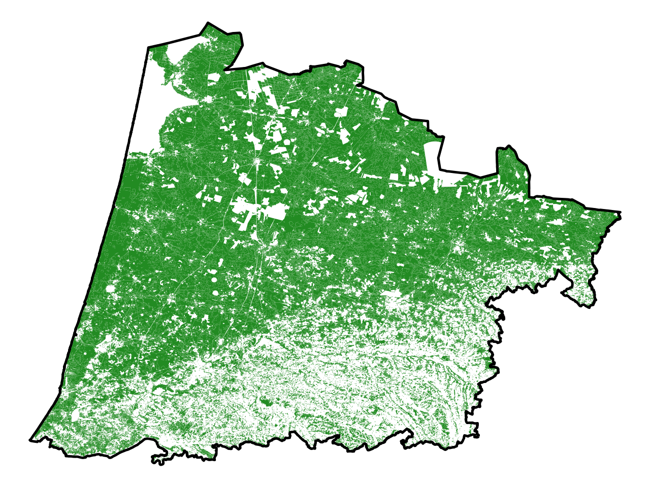
Here, the map is quite clear and conveys a relatively readable message. Of course, it does not provide details that might interest curious viewers (e.g., which specific localities are particularly forested), but it does offer a synthetic view of the studied phenomenon.
The previous exercise allowed us to create a solid color map. This naturally leads us to choropleth maps, where color shading is used to represent socioeconomic information.
We will use population data available from the datasets retrieved via cartiflette2. As an exercise, we will create a choropleth map styled in a vintage look, reminiscent of the early maps of Dupin (1826).
The goal of this exercise is to enhance the information presented on the departmental map.
Quickly generate a map of the departments, coloring them according to the POPULATION variable.
This map presents several issues:
The next questions aim to improve this step by step.
Recreate this map using the Lambert 93 projection.
Discretize the POPULATION variable into 4 classes using quantile-based discretization, then recreate the map.
Normalize the population by the area of each department (in km²) by creating a new variable using .area.div(1e6)3.
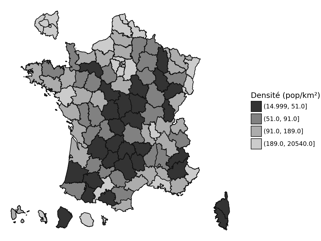
Choose a vintage grayscale color palette.
The first question produces a map that looks like this:
It is already improved by using a projection suited for the territory, Lambert 93 (question 2):
The map below, after discretization (question 3), already provides a more accurate representation of population inequalities. We can see the “diagonal of emptiness” starting to emerge, which is expected in a population map.
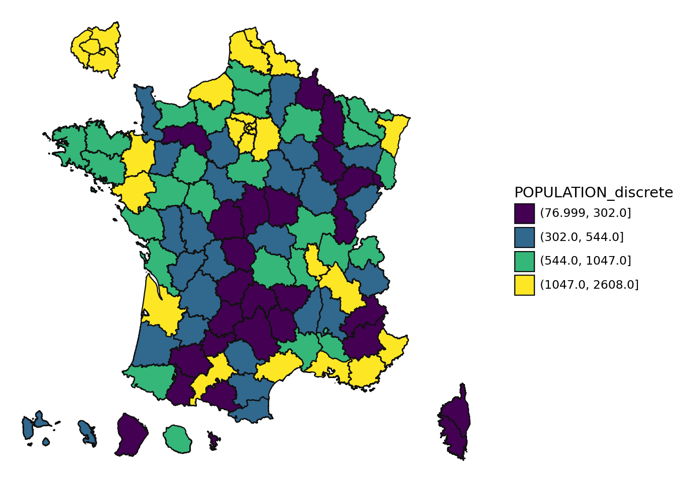
However, one of the problems with choropleth maps is that they give disproportionate visual weight to large areas. This issue was particularly highlighted in election maps with the visual “Land doesn’t vote, people do” (see the 2024 European elections version).
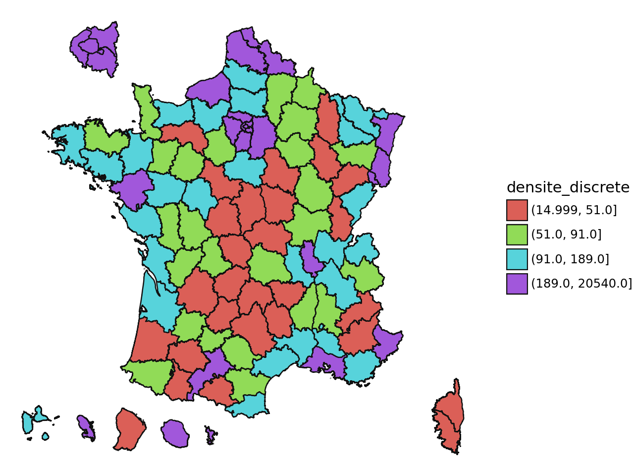
While we cannot completely eliminate this issue—doing so would require switching to a different type of visualization, such as proportional circles—we can mitigate the effect of area on our variable of interest by representing density (population per km² rather than total population).
We obtain the following map when representing population density instead of total population:
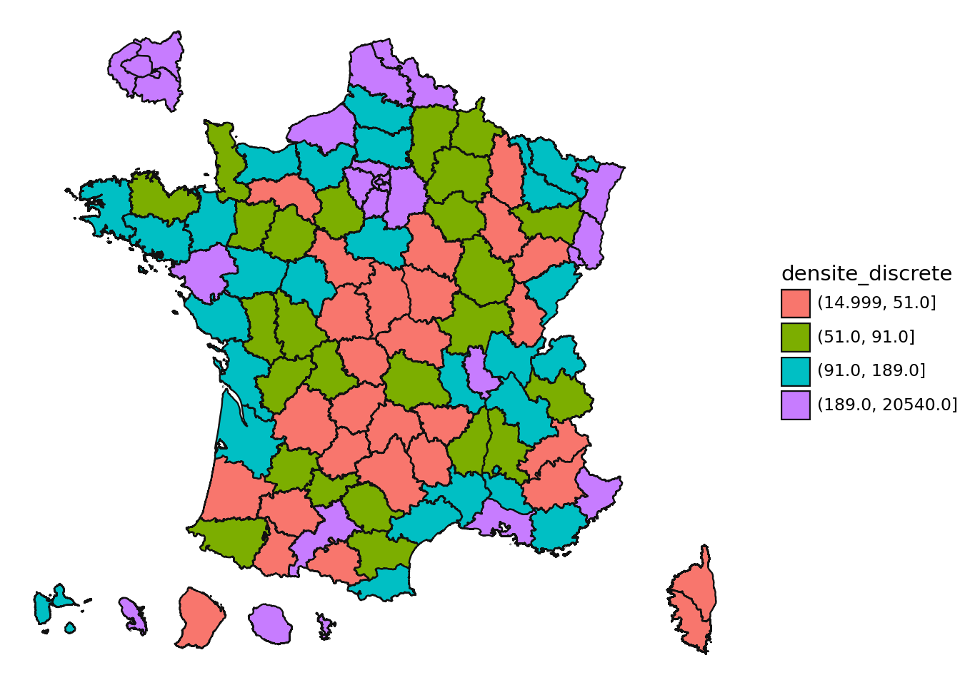
This already provides a more accurate picture of population distribution across France. However, the default desigual color palette does not help much in capturing the nuances. Using a gradient color palette, which considers the ordinal nature of our data, results in a more readable map (question 5):
This is already better. However, to create an even more effective map, a more suitable discretization method should be chosen. This is an important iterative process that requires multiple skill sets, including statistics, sociology or economics (depending on the type of information represented), and computer science. In short, the typical skill set of a data scientist.
Until now, we have worked with data where simply displaying administrative boundaries was sufficient for context. Now, let’s focus on a case where having a contextual basemap becomes crucial: sub-municipal maps.
For this, we will represent the locations of Vélib’ stations. These are available as open data from the Paris City Hall website.
Velib station location dataset is available from Paris opendata portal as a GeoJSON file:
import geopandas as gpd
velib_data = "https://opendata.paris.fr/explore/dataset/velib-emplacement-des-stations/download/?format=geojson&timezone=Europe/Berlin&lang=fr"
stations = gpd.read_file(velib_data)
stations.head(2)| capacity | stationcode | coordonnees_geo | name | geometry | |
|---|---|---|---|---|---|
| 0 | 28 | 40001 | [48.798922410229, 2.4537451531298] | Hôpital Mondor | POINT (2.45375 48.79892) |
| 1 | 22 | 25006 | [48.862453313908, 2.1961666225454] | Place Nelson Mandela | POINT (2.19617 48.86245) |
Administrative borders are going to be useful. Here is a snippet to retrieve them:
from cartiflette import carti_download
# 1. Fonds communaux
contours_villes_arrt = carti_download(
values = ["75", "92", "93", "94"],
crs = 4326,
borders="COMMUNE_ARRONDISSEMENT",
filter_by="DEPARTEMENT",
source="EXPRESS-COG-CARTO-TERRITOIRE",
year=2022)
# 2. Départements
departements = contours_villes_arrt.dissolve("INSEE_DEP")plot method. Can you determine where they are?MarkerCluster feature in Folium to create an interactive map.If we directly plot stations using the plot method, we lack context:
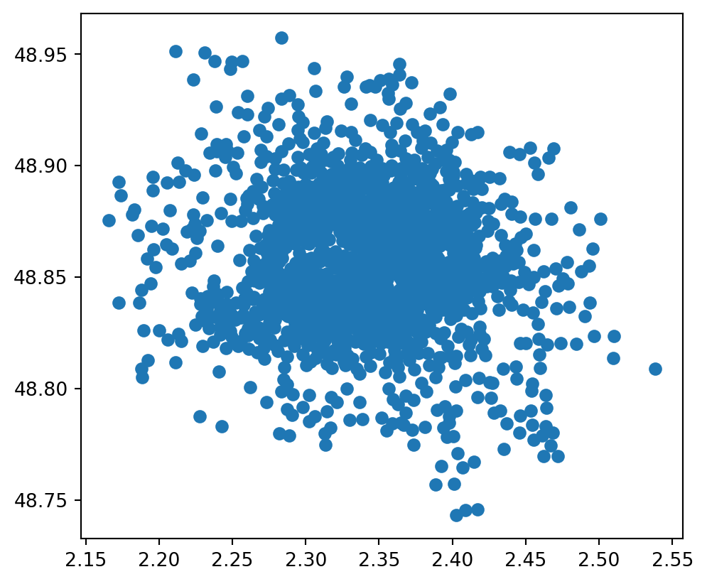
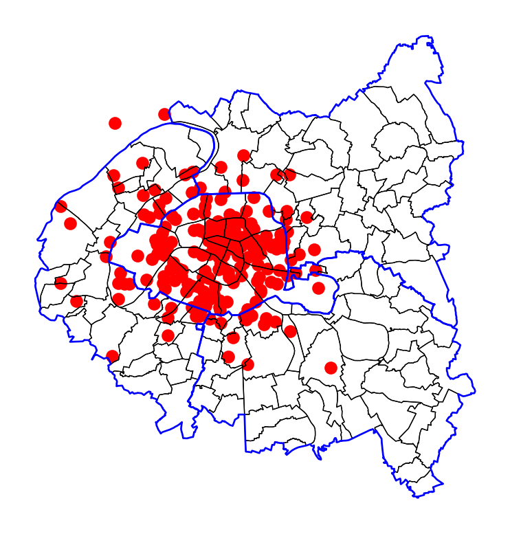
It is even impossible to determine whether we are actually in Paris. We can attempt to associate our data with administrative boundaries to confirm that we are indeed in the Paris region.
The first step is to retrieve the boundaries of Parisian districts and neighboring municipalities, which can be easily done using cartiflette:
If we now use administrative areas mask to provide context, we can be reassured about the nature of the data.
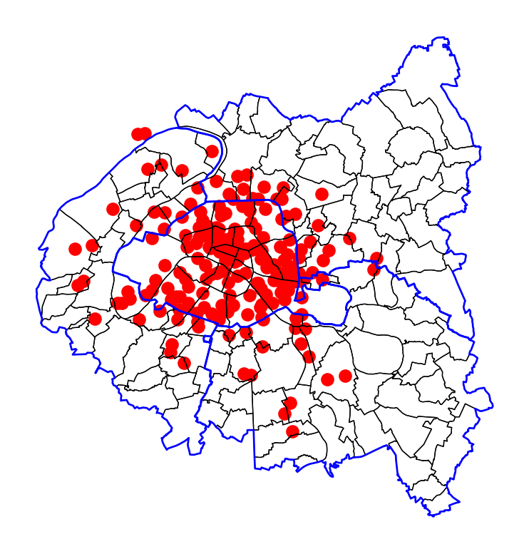
Parisians will easily recognize their city because they are familiar with the spatial organization of this metropolitan area. However, for readers unfamiliar with it, this map will be of little help. The ideal solution is to use Folium’s contextual basemap.
To avoid cluttering the map, it is useful to leverage Folium’s interactive features, allowing the user to navigate the map and display an appropriate amount of information based on the visible window. For this, Folium includes a very handy MarkerCluster functionality.
Thus, we can create the desired map as follows:
This site was built automatically through a Github action using the Quarto
The environment used to obtain the results is reproducible via uv. The pyproject.toml file used to build this environment is available on the linogaliana/python-datascientist repository
pyproject.toml
[project]
name = "python-datascientist"
version = "0.1.0"
description = "Source code for Lino Galiana's Python for data science course"
readme = "README.md"
requires-python = ">=3.13,<3.14"
dependencies = [
"altair>=6.0.0",
"cartiflette",
"contextily==1.6.2",
"duckdb>=0.10.1",
"folium>=0.19.6",
"gdal==3.11.4",
"graphviz==0.20.3",
"great-tables>=0.12.0",
"gt-extras>=0.0.8",
"ipykernel>=6.29.5",
"jupyter>=1.1.1",
"jupyter-cache>=1.0.0",
"kaleido>=0.2.1",
"langchain-community>=0.3.27",
"loguru==0.7.3",
"markdown>=3.8",
"nbclient>=0.10.0",
"nbformat>=5.10.4",
"nltk>=3.9.1",
"pandas>=2.3.3",
"pip>=25.1.1",
"plotly>=6.1.2",
"plotnine>=0.15",
"polars>=1.8.2",
"pyarrow>=17.0.0",
"pynsee>=0.1.8",
"python-dotenv>=1.0.1",
"python-frontmatter>=1.1.0",
"pywaffle>=1.1.1",
"requests>=2.32.3",
"scikit-image>=0.24.0",
"scikit-learn>=1.8.0",
"scipy>=1.13.0",
"seaborn>=0.13.2",
"selenium<4.39.0",
"spacy>=3.8.4",
"webdriver-manager>=4.0.2",
"wordcloud==1.9.3",
]
[tool.uv.sources]
cartiflette = { git = "https://github.com/inseefrlab/cartiflette" }
gdal = [
{ index = "gdal-wheels", marker = "sys_platform == 'linux'" },
{ index = "geospatial_wheels", marker = "sys_platform == 'win32'" },
]
[[tool.uv.index]]
name = "geospatial_wheels"
url = "https://nathanjmcdougall.github.io/geospatial-wheels-index/"
explicit = true
[[tool.uv.index]]
name = "gdal-wheels"
url = "https://gitlab.com/api/v4/projects/61637378/packages/pypi/simple"
explicit = true
[dependency-groups]
dev = [
"nb-clean>=4.0.1",
]
To use exactly the same environment (version of Python and packages), please refer to the documentation for uv.
| SHA | Date | Author | Description |
|---|---|---|---|
| f250c24f | 2025-12-13 19:15:02 | Lino Galiana | Un essai d’histogramme en légende (#661) |
| c3d51646 | 2025-08-12 17:28:51 | Lino Galiana | Ajoute un résumé au début de chaque chapitre (première partie) (#634) |
| 94648290 | 2025-07-22 18:57:48 | Lino Galiana | Fix boxes now that it is better supported by jupyter (#628) |
| 91431fa2 | 2025-06-09 17:08:00 | Lino Galiana | Improve homepage hero banner (#612) |
| 26226eea | 2025-01-31 17:54:48 | lgaliana | Chapitre cartographie en anglais |
| cbe6459f | 2024-11-12 07:24:15 | lgaliana | Revoir quelques abstracts |
| 886389c4 | 2024-10-21 08:59:14 | lgaliana | rappel mercator folium |
| 9cf2bde5 | 2024-10-18 15:49:47 | lgaliana | Reconstruction complète du chapitre de cartographie |
| d2422572 | 2024-08-22 18:51:51 | Lino Galiana | At this point, notebooks should now all be functional ! (#547) |
| 06d003a1 | 2024-04-23 10:09:22 | Lino Galiana | Continue la restructuration des sous-parties (#492) |
| 8c316d0a | 2024-04-05 19:00:59 | Lino Galiana | Fix cartiflette deprecated snippets (#487) |
| ce33d5dc | 2024-01-16 15:47:22 | Lino Galiana | Adapte les exemples de code de cartiflette (#482) |
| 005d89b8 | 2023-12-20 17:23:04 | Lino Galiana | Finalise l’affichage des statistiques Git (#478) |
| 3fba6124 | 2023-12-17 18:16:42 | Lino Galiana | Remove some badges from python (#476) |
| 4cd44f35 | 2023-12-11 17:37:50 | Antoine Palazzolo | Relecture NLP (#474) |
| 1f23de28 | 2023-12-01 17:25:36 | Lino Galiana | Stockage des images sur S3 (#466) |
| b68369d4 | 2023-11-18 18:21:13 | Lino Galiana | Reprise du chapitre sur la classification (#455) |
| 09654c71 | 2023-11-14 15:16:44 | Antoine Palazzolo | Suggestions Git & Visualisation (#449) |
| 889a71ba | 2023-11-10 11:40:51 | Antoine Palazzolo | Modification TP 3 (#443) |
| ad654c5f | 2023-10-10 14:23:05 | linogaliana | CQuick fix gzip csv |
| 1c646606 | 2023-10-04 15:52:52 | Lino Galiana | Quick fix remove contextily (#420) |
| 154f09e4 | 2023-09-26 14:59:11 | Antoine Palazzolo | Des typos corrigées par Antoine (#411) |
| c7f8c941 | 2023-09-01 09:27:43 | Lino Galiana | Ajoute un champ citation (#403) |
| 17a238f2 | 2023-08-30 15:06:18 | Lino Galiana | Nouvelles données compteurs (#402) |
| 0035b743 | 2023-08-29 14:51:26 | Lino Galiana | Temporary fix for cartography pipeline (#401) |
| a8f90c2f | 2023-08-28 09:26:12 | Lino Galiana | Update featured paths (#396) |
| 3bdf3b06 | 2023-08-25 11:23:02 | Lino Galiana | Simplification de la structure 🤓 (#393) |
| 78ea2cbd | 2023-07-20 20:27:31 | Lino Galiana | Change titles levels (#381) |
| 8df7cb22 | 2023-07-20 17:16:03 | linogaliana | Change link |
| f0c583c0 | 2023-07-07 14:12:22 | Lino Galiana | Images viz (#371) |
| f21a24d3 | 2023-07-02 10:58:15 | Lino Galiana | Pipeline Quarto & Pages 🚀 (#365) |
| 38693f62 | 2023-04-19 17:22:36 | Lino Galiana | Rebuild visualisation part (#357) |
| 32486330 | 2023-02-18 13:11:52 | Lino Galiana | Shortcode rawhtml (#354) |
| b0abd027 | 2022-12-12 07:57:22 | Lino Galiana | Fix cartiflette in additional exercise (#334) |
| e56f6fd5 | 2022-12-03 17:00:55 | Lino Galiana | Corrige typos exo compteurs (#329) |
| f10815b5 | 2022-08-25 16:00:03 | Lino Galiana | Notebooks should now look more beautiful (#260) |
| 494a85ae | 2022-08-05 14:49:56 | Lino Galiana | Images featured ✨ (#252) |
| d201e3cd | 2022-08-03 15:50:34 | Lino Galiana | Pimp la homepage ✨ (#249) |
| 5698e303 | 2022-06-03 18:28:37 | Lino Galiana | Finalise widget (#232) |
| 7b9f27be | 2022-06-03 17:05:15 | Lino Galiana | Essaie régler les problèmes widgets JS (#231) |
| 12965bac | 2022-05-25 15:53:27 | Lino Galiana | :launch: Bascule vers quarto (#226) |
| 9c71d6e7 | 2022-03-08 10:34:26 | Lino Galiana | Plus d’éléments sur S3 (#218) |
| 66a52761 | 2021-11-23 16:13:20 | Lino Galiana | Relecture partie visualisation (#181) |
| 2a8809fb | 2021-10-27 12:05:34 | Lino Galiana | Simplification des hooks pour gagner en flexibilité et clarté (#166) |
| 2f4d3905 | 2021-09-02 15:12:29 | Lino Galiana | Utilise un shortcode github (#131) |
| 2e4d5862 | 2021-09-02 12:03:39 | Lino Galiana | Simplify badges generation (#130) |
| 4cdb759c | 2021-05-12 10:37:23 | Lino Galiana | :sparkles: :star2: Nouveau thème hugo :snake: :fire: (#105) |
| 7f9f97bc | 2021-04-30 21:44:04 | Lino Galiana | 🐳 + 🐍 New workflow (docker 🐳) and new dataset for modelization (2020 🇺🇸 elections) (#99) |
| 29242152 | 2020-10-08 13:35:18 | Lino Galiana | modif slug cartographie |
| 64776878 | 2020-10-08 13:31:00 | Lino Galiana | Visualisation cartographique (#68) |
This calculation is possible because both datasets are in the Lambert 93 projection, which allows for geometric operations (including surface area calculations).↩︎
Stricto sensu, we should verify that these columns accurately correspond to the official population counts defined by Insee. This variable is natively provided by IGN in its basemap data. We leave this verification to interested readers, as it offers a good opportunity to practice Pandas skills.↩︎
Lambert 93 provides area in square meters. To convert it to km², use div(1e6).↩︎
@book{galiana2025,
author = {Galiana, Lino},
title = {Python Pour La Data Science},
date = {2025},
url = {https://pythonds.linogaliana.fr/},
doi = {10.5281/zenodo.8229676},
langid = {en}
}