import numpy as np
import pandas as pd
import matplotlib.pyplot as pltIf you want to try the examples in this tutorial:

TipSkills to be acquired by the end of this chapter
- Import a dataset as a
Pandasdataframe and explore its structure; - Perform manipulations on columns and rows;
- Construct aggregate statistics and chain operations;
- Use
Pandasgraphical methods to quickly represent data distribution.
1 Introduction
The Pandas package has been the central piece of the data science ecosystem for about a decade. The DataFrame, a central object in languages like R or Stata, had long been absent in the Python ecosystem. Yet, thanks to Numpy, all the basic components were present but needed to be reconfigured to meet the needs of data scientists.
Wes McKinney, when he built Pandas to provide a dataframe leveraging the numerical computation library Numpy in the background, enabled a significant leap forward for Python in data analysis, explaining its popularity in the data science ecosystem. Pandas is not without limitations1, which we will have the opportunity to discuss, but the vast array of analysis methods it offers greatly simplifies data analysis work. For more information on this package, the reference book by McKinney (2012) presents many of the package’s features.
In this chapter, we will focus on the most relevant elements in the context of an introduction to data science, leaving interested users to deepen their knowledge with the abundant resources available on the subject.
As datasets generally gain value by associating multiple sources, for example, to relate a record to contextual data or to link two client databases to obtain meaningful data, the next chapter will present how to merge different datasets with Pandas. By the end of the next chapter, thanks to data merging, we will have a detailed database on the carbon footprints of the French2.
1.1 Data used in this chapter
In this Pandas tutorial, we will use:
- Greenhouse gas emissions estimated at the municipal level by ADEME. The dataset is available on data.gouv and can be queried directly in
Pythonwith this URL.
The next chapter will allow us to apply the elements presented in this chapter with the above data combined with contextual data at the municipal level.
1.2 Environment
We will follow the usual conventions in importing packages:
To obtain reproducible results, you can set the seed of the pseudo-random number generator.
np.random.seed(123)Throughout this demonstration of the main Pandas functionalities, and in the next chapter, I recommend regularly referring to the following resources:
- The official
Pandasdocumentation, especially the language comparison page, which is very useful; - This tutorial, designed for users of
Observable Javascript, but offering many interesting examples forPandasaficionados; - The following cheatsheet from this post.
As a reminder, to execute the code examples in an interactive notebook, you can use the shortcuts at the top of the page to launch it in your preferred environment.
2 Pandas logic
2.1 Anatomy of a Pandas table
The central object in the Pandas logic is the DataFrame. It is a special data structure with two dimensions, structured by aligning rows and columns. Unlike a matrix, columns can be of different types.
A DataFrame consists of the following elements:
- the row index;
- the column name;
- the data value;

Pandas DataFrame, borrowed from https://x.com/epfl_exts/status/9975060006000844802.2 Before seeing DataFrame, we need to know Pandas Series
In fact, a DataFrame is a collection of objects called pandas.Series. These Series are one-dimensional objects that are extensions of the one-dimensional Numpy arrays3. In particular, to facilitate the handling of categorical or temporal data, additional variable types are available in Pandas compared to Numpy (categorical, datetime64, and timedelta64). These types are associated with optimized methods to facilitate the processing of this data.
There are several possible types for a pandas.Series, extending the basic data types in Python, which will determine the behavior of this variable. Indeed, many operations do not have the same meaning depending on whether the value is numeric or not.
The simplest types (int or float) correspond to numeric values:
poids = pd.Series(
    [3, 7, 12]
)
poids
0 3
1 7
2 12
dtype: int64
ImportantMissing Values are tricky !
In general, if Pandas exclusively detects integer values in a variable, it will use the int type to optimize memory. This choice makes sense. However, it has a drawback: Numpy, and therefore by extension Pandas, cannot represent missing values for the int type (more on missing values below).
Pending the shift to Arrow, which can handle missing values in int, the method to use is to convert to the float type if the variable will have missing values, which is quite simple:
For textual data, it is just as simple:
animal = pd.Series(
  ['chat', 'chien', 'koala']
)
animal
0 chat
1 chien
2 koala
dtype: strSince Pandas 3.0, exclusively textual data natively receives the dedicated str type, as shown above: object is no longer the default type used for text. The object type remains a catch-all, but it is now reserved for genuinely mixed data (text and numbers, or arbitrary Python objects, type mixed). Historically, object acted as an intermediate type between the factor and character of R; this role is now better served by the str/category distinction. There is indeed an equivalent type to factor in Pandas, the category type, to be preferred when a variable has a finite and relatively small list of possible values (bringing memory and performance gains). It is therefore recommended, when focusing on a low-cardinality textual variable, to convert it explicitly:
- 1
-
Pour convertir en
category(le choix qui fait sens ici) - 2
-
Pour repasser en
strexplicitement (redondant ici puisque c’est déjà le type par défaut depuisPandas3.0, mais utile si la colonne provient d’un import ayant forcé un typageobject)
0     chat
1    chien
2    koala
dtype: strIt is important to examine the types of your Pandas objects and convert them if they do not make sense; Pandas makes optimized choices, but it may be necessary to correct them because Pandas does not know your future data usage. This is one of the tasks to do during feature engineering, the set of steps for preparing data for future use.
3 From Series to DataFrame
We have created two independent series, animal and poids, which are related. In the matrix world, this would correspond to moving from a vector to a matrix. In the Pandas world, this means moving from a Series to a DataFrame.
This is done naturally with Pandas:
animaux = pd.DataFrame(
  zip(animal, poids),
  columns = ['animal','poids']
)
animaux| animal | poids | |
|---|---|---|
| 0 | chat | 3 |
| 1 | chien | 7 |
| 2 | koala | 12 |
- We need to use
ziphere becausePandasexpects a structure like{"var1": [val1, val2], "var2": [val1, val2]}, which is not what we prepared previously. However, we will see that this approach is not the most common for creating aDataFrame.
The essential difference between a Series and a Numpy object is indexing. In Numpy, indexing is implicit; it allows accessing data (the one at the index located at position i). With a Series, you can, of course, use a positional index, but more importantly, you can use more explicit indices.
This allows accessing data more naturally, using column names, for example:
animaux['poids']0 3
1 7
2 12
Name: poids, dtype: int64The existence of an index makes subsetting, that is, selecting rows or columns, particularly easy. DataFrames have two indices: those for rows and those for columns. You can make selections on both dimensions. Anticipating later exercises, you can see that this will facilitate row selection:
animaux.loc[animaux['animal'] == "chat", 'poids']0 3
Name: poids, dtype: int64This instruction is equivalent to the SQL command:
SELECT poids FROM animaux WHERE animal == "chat"If we return to our animaux dataset, we can see the row number displayed on the left:
animaux| animal | poids | |
|---|---|---|
| 0 | chat | 3 |
| 1 | chien | 7 |
| 2 | koala | 12 |
This is the default index for the row dimension because we did not configure one. It is not mandatory; it is quite possible to have an index corresponding to a variable of interest (we will discover this when we explore groupby in the next chapter). However, this can be tricky, and it is recommended that this be only transitory, hence the importance of regularly performing reset_index.
3.1 The concept of tidy data
The concept of tidy data, popularized by Hadley Wickham through his R packages (see Wickham, Çetinkaya-Rundel, and Grolemund (2023)), is highly relevant for describing the structure of a Pandas DataFrame. The three rules of tidy data are as follows:
- Each variable has its own column;
- Each observation has its own row;
- A value, representing an observation of a variable, is located in a single cell.

These principles may seem like common sense, but you will find that many data formats do not adhere to them. For example, Excel spreadsheets often have values spanning multiple columns or several merged rows. Restructuring this data according to the tidy data principle will be crucial to performing analysis on it.
4 Importing Data with Pandas
If you had to manually create all your DataFrames from vectors, Pandas would not be practical. Pandas offers many functions to read data stored in different formats.
The simplest data to read are tabular data stored in an appropriate format. The two main formats to know are CSV and Parquet. The former has the advantage of simplicity - it is universal, known to all, and readable by any text editor. The latter is gaining popularity in the data ecosystem because it addresses some limitations of CSV (optimized storage, predefined variable types…) but has the disadvantage of not being readable without a suitable tool (which fortunately are increasingly present in standard code editors like VSCode). For more information on the difference between CSV and Parquet, refer to the deep dive chapters on the subject.
Data stored in other text-derived formats from CSV (.txt, .tsv…) or formats like JSON are readable with Pandas, but sometimes it takes a bit of iteration to find the correct reading parameters. In other chapters, we will discover that other data formats related to different data structures are also readable with Python.
Flat formats (.csv, .txt…) and the Parquet format are easy to use with Pandas because they are not proprietary and they store data in a tidy form. Data from spreadsheets, Excel or LibreOffice, are more or less complicated to import depending on whether they follow this schema or not. This is because these tools are used indiscriminately. While in the data science world, they should primarily be used to disseminate final tables for reporting, they are often used to disseminate raw data that could be better shared through more suitable channels.
One of the main difficulties with spreadsheets is that the data are usually associated with documentation in the same tab - for example, the spreadsheet has some lines describing the sources before the table - which requires human intelligence to assist Pandas during the import phase. This will always be possible, but when there is an alternative in the form of a flat file, there should be no hesitation.
4.1 Reading Data from a Local Path
This exercise aims to demonstrate the benefit of using a relative path rather than an absolute path to enhance code reproducibility. However, we will later recommend reading directly from the internet when possible and when it does not involve the recurrent download of a large file.
To prepare for this exercise, the following code will allow you to download data and write it locally:
import requests

url = "https://www.insee.fr/fr/statistiques/fichier/6800675/v_commune_2023.csv"
url_backup = "https://minio.lab.sspcloud.fr/lgaliana/data/python-ENSAE/cog_2023.csv"

try:
    response = requests.get(url)
except requests.exceptions.RequestException as e:
    print(f"Error : {e}")
    response = requests.get(url_backup)

# Only download if one of the request succeeded
if response.status_code == 200:
    with open("cog_2023.csv", "wb") as file:
        file.write(response.content)
TipPreliminary Exercise: Importing a CSV (Optional)
- Use the code above ☝️ to download the data. Use
Pandasto read the downloaded file. - Find where the data was written. Observe the structure of this directory.
- Create a new folder using the file explorer (on the left in
JupyterorVSCode). Move the CSV and the notebook. Restart the kernel and adjust your code if needed. Repeat this process several times with different folders. What issues might you encounter?
| TYPECOM | COM | REG | DEP | CTCD | ARR | TNCC | NCC | NCCENR | LIBELLE | CAN | COMPARENT | |
|---|---|---|---|---|---|---|---|---|---|---|---|---|
| 0 | COM | 01001 | 84.0 | 01 | 01D | 012 | 5 | ABERGEMENT CLEMENCIAT | Abergement-Clémenciat | L'Abergement-Clémenciat | 0108 | NaN |
| 1 | COM | 01002 | 84.0 | 01 | 01D | 011 | 5 | ABERGEMENT DE VAREY | Abergement-de-Varey | L'Abergement-de-Varey | 0101 | NaN |
The main issue with reading from files stored locally is the risk of becoming dependent on a file system that is not necessarily shared. It is better, whenever possible, to directly read the data with an HTTPS link, which Pandas can handle. Moreover, when working with open data, this ensures that you are using the latest available data and not a local duplication that may not be up to date.
4.2 Reading from a CSV Available on the Internet
The URL to access the data can be stored in an ad hoc variable:
url = "https://koumoul.com/s/data-fair/api/v1/datasets/igt-pouvoir-de-rechauffement-global/convert"The goal of the next exercise is to get familiar with importing and displaying data using Pandas and displaying a few observations.
TipExercise 1: Importing a CSV and Exploring Data Structure
- Import the data from Ademe using the
Pandaspackage and the dedicated command for importing CSVs. Name the obtainedDataFrameemissions4. - Use the appropriate methods to display the first 10 values, the last 15 values, and a random sample of 10 values using the appropriate methods from the
Pandaspackage. - Draw 5 percent of the sample without replacement.
- Keep only the first 10 rows and randomly draw from these to obtain a DataFrame of 100 data points.
- Make 100 draws from the first 6 rows with a probability of 1/2 for the first observation and a uniform probability for the others.
If you get stuck on question 1
Read the documentation for read_csv (very well done) or look for examples online to discover this function.
As illustrated by this exercise, displaying DataFrames in notebooks is quite ergonomic. The first and last rows are displayed automatically. For valuation tables present in a report or research article, the next chapter introduces great_tables, which offers very rich table formatting features.
WarningWarning
Be careful with display and commands that reveal data (head, tail, etc.) in a notebook that handles confidential data when using version control software like Git (see dedicated chapters).
Indeed, you may end up sharing data inadvertently in the Git history. As explained in the chapter dedicated to Git, a file named .gitignore is sufficient to create some rules to avoid unintentional sharing of data with Git.
5 Exploring the Structure of a DataFrame
Pandas offers a data schema quite familiar to users of statistical software like R. Similar to the main data processing paradigms like the tidyverse (R), the grammar of Pandas inherits from SQL logic. The philosophy is very similar: operations are performed to select rows, columns, sort rows based on column values, apply standardized treatments to variables, etc. Generally, operations that reference variable names are preferred over those that reference row or column numbers.
Whether you are familiar with SQL or R, you will find a similar logic to what you know, although the names might differ: df.loc[df['y']=='b'] may be written as df %>% filter(y=='b') (R) or SELECT * FROM df WHERE y == 'b' (SQL), but the logic is the same.
Pandas offers a plethora of pre-implemented functionalities. It is highly recommended, before writing a function, to consider if it is natively implemented in Numpy, Pandas, etc. Most of the time, if a solution is implemented in a library, it should be used as it will be more efficient than what you would implement.
To present the most practical methods for data analysis, we can use the example of the municipal CO2 consumption data from Ademe, which was the focus of the previous exercises.
df = pd.read_csv("https://koumoul.com/s/data-fair/api/v1/datasets/igt-pouvoir-de-rechauffement-global/convert")
df| INSEE commune | Commune | Agriculture | Autres transports | Autres transports international | CO2 biomasse hors-total | Déchets | Energie | Industrie hors-énergie | Résidentiel | Routier | Tertiaire | |
|---|---|---|---|---|---|---|---|---|---|---|---|---|
| 0 | 01001 | L'ABERGEMENT-CLEMENCIAT | 3711.425991 | NaN | NaN | 432.751835 | 101.430476 | 2.354558 | 6.911213 | 309.358195 | 793.156501 | 367.036172 |
| 1 | 01002 | L'ABERGEMENT-DE-VAREY | 475.330205 | NaN | NaN | 140.741660 | 140.675439 | 2.354558 | 6.911213 | 104.866444 | 348.997893 | 112.934207 |
| 2 | 01004 | AMBERIEU-EN-BUGEY | 499.043526 | 212.577908 | NaN | 10313.446515 | 5314.314445 | 998.332482 | 2930.354461 | 16616.822534 | 15642.420313 | 10732.376934 |
| 3 | 01005 | AMBERIEUX-EN-DOMBES | 1859.160954 | NaN | NaN | 1144.429311 | 216.217508 | 94.182310 | 276.448534 | 663.683146 | 1756.341319 | 782.404357 |
| 4 | 01006 | AMBLEON | 448.966808 | NaN | NaN | 77.033834 | 48.401549 | NaN | NaN | 43.714019 | 398.786800 | 51.681756 |
| ... | ... | ... | ... | ... | ... | ... | ... | ... | ... | ... | ... | ... |
| 35793 | 95676 | VILLERS-EN-ARTHIES | 1628.065094 | NaN | NaN | 165.045396 | 65.063617 | 11.772789 | 34.556067 | 176.098160 | 309.627908 | 235.439109 |
| 35794 | 95678 | VILLIERS-ADAM | 698.630772 | NaN | NaN | 1331.126598 | 111.480954 | 2.354558 | 6.911213 | 1395.529811 | 18759.370071 | 403.404815 |
| 35795 | 95680 | VILLIERS-LE-BEL | 107.564967 | NaN | NaN | 8367.174532 | 225.622903 | 534.484607 | 1568.845431 | 22613.830247 | 12217.122402 | 13849.512001 |
| 35796 | 95682 | VILLIERS-LE-SEC | 1090.890170 | NaN | NaN | 326.748418 | 108.969749 | 2.354558 | 6.911213 | 67.235487 | 4663.232127 | 85.657725 |
| 35797 | 95690 | WY-DIT-JOLI-VILLAGE | 1495.103542 | NaN | NaN | 125.236417 | 97.728612 | 4.709115 | 13.822427 | 117.450851 | 504.400972 | 147.867245 |
35798 rows × 12 columns
5.1 Dimensions and Structure of a DataFrame
The first useful methods allow displaying some attributes of a DataFrame.
df.axes[RangeIndex(start=0, stop=35798, step=1),
Index(['INSEE commune', 'Commune', 'Agriculture', 'Autres transports',
       'Autres transports international', 'CO2 biomasse hors-total', 'Déchets',
       'Energie', 'Industrie hors-énergie', 'Résidentiel', 'Routier',
       'Tertiaire'],
dtype='str')]df.columnsIndex(['INSEE commune', 'Commune', 'Agriculture', 'Autres transports',
'Autres transports international', 'CO2 biomasse hors-total', 'Déchets',
'Energie', 'Industrie hors-énergie', 'Résidentiel', 'Routier',
'Tertiaire'],
dtype='str')df.indexRangeIndex(start=0, stop=35798, step=1)5.2 Dimensions and Structure of a DataFrame
The first useful methods allow displaying some attributes of a DataFrame.
df.ndim2df.shape(35798, 12)df.size429576To know the dimensions of a DataFrame, some practical methods can be used:
df.ndim2df.shape(35798, 12)df.size429576To determine the number of unique values of a variable, rather than writing a function yourself, use the nunique method. For example,
df['Commune'].nunique()33338Pandas offers many useful methods. Here is a summary of those related to data structure, accompanied by a comparison with R:
| Operation | pandas | dplyr (R) |
|---|---|---|
| Retrieve column names | df.columns |
colnames(df) |
| Retrieve dimensions | df.shape |
dim(df) |
| Retrieve unique values of a variable | df['myvar'].nunique() |
df %>% summarise(distinct(myvar)) |
5.3 Accessing elements of a DataFrame
In SQL, performing operations on columns is done with the SELECT command. With Pandas, to access an entire column, several approaches can be used:
dataframe.variable, for exampledf.Energie. This method requires column names without spaces or special characters, which excludes many real datasets. It is not recommended.dataframe[['variable']]to return the variable as aDataFrame. This method can be tricky for a single variable; it’s better to usedataframe.loc[:,['variable']], which is more explicit about the nature of the resulting object.dataframe['variable']to return the variable as aSeries. For example,df[['Autres transports']]ordf['Autres transports']. This is the preferred method.
To retrieve multiple columns at once, there are two approaches, with the second being preferable:
dataframe[['variable1', 'variable2']]dataframe.loc[:, ['variable1', 'variable2']]
This is equivalent to SELECT variable1, variable2 FROM dataframe in SQL.
Using .loc may seem excessively verbose, but it ensures that you are performing a subset operation on the column dimension. DataFrames have two indices, for rows and columns, and implicit operations can sometimes cause surprises, so it’s more reliable to be explicit.
5.4 Accessing rows
To access one or more values in a DataFrame, there are two recommended methods, depending on the form of the row or column indices used:
df.iloc: uses indices. This method is somewhat unreliable because a DataFrame’s indices can change during processing (especially when performing group operations).df.loc: uses labels. This method is recommended.
WarningWarning
Code snippets using the df.ix structure should be avoided as the function is deprecated and may disappear at any time.
iloc refers to the indexing from 0 to N, where N equals df.shape[0] of a pandas.DataFrame. loc refers to the values of df’s index. For example, with the pandas.DataFrame df_example:
df_example = pd.DataFrame(
    {'month': [1, 4, 7, 10], 'year': [2012, 2014, 2013, 2014], 'sale': [55, 40, 84, 31]})
df_example = df_example.set_index('month')
df_example| year | sale | |
|---|---|---|
| month | ||
| 1 | 2012 | 55 |
| 4 | 2014 | 40 |
| 7 | 2013 | 84 |
| 10 | 2014 | 31 |
df_example.loc[1, :]will return the first row ofdf(row where themonthindex equals 1);df_example.iloc[1, :]will return the second row (since Python indexing starts at 0);df_example.iloc[:, 1]will return the second column, following the same principle.
Later exercises will allow practicing this syntax on our dataset of carbon emissions.
6 Main data wrangling routine
The most frequent operations in SQL are summarized in the following table. It is useful to know them (many data manipulation syntaxes use these terms) because, one way or another, they cover most data manipulation uses. We will describe some of them later:
| Operation | SQL | pandas | dplyr (R) |
|---|---|---|---|
| Select variables by name | SELECT |
df.loc[:, ['Autres transports','Energie']] |
df %>% select(Autres transports, Energie) |
| Select observations based on one or more conditions | FILTER |
df.loc[pd.col('Agriculture')>2000] |
df %>% filter(Agriculture>2000) |
| Sort the table by one or more variables | SORT BY |
df.sort_values(['Commune','Agriculture']) |
df %>% arrange(Commune, Agriculture) |
| Add variables that are functions of other variables | SELECT *, LOG(Agriculture) AS x FROM df |
df = df.assign(x = np.log(pd.col('Agriculture'))) |
df %>% mutate(x = log(Agriculture)) |
The next chapters will let us go further by adding other, more complex operations (joins, group-by statistics, etc.)
6.1 Operations on Columns: Adding or Removing Variables, Renaming Them, etc.
Technically, Pandas DataFrames are mutable objects in the Python language, meaning it is possible to change the DataFrame as needed during processing.
The most classic operation is adding or removing variables to the data table. The simplest way to add columns is by reassignment. For example, to create a dep variable that corresponds to the first two digits of the commune code (INSEE code), simply take the variable and apply the appropriate treatment (in this case, keep only its first two characters):
df['dep'] = df['INSEE commune'].str[:2]
df.head(3)| INSEE commune | Commune | Agriculture | Autres transports | Autres transports international | CO2 biomasse hors-total | Déchets | Energie | Industrie hors-énergie | Résidentiel | Routier | Tertiaire | dep | |
|---|---|---|---|---|---|---|---|---|---|---|---|---|---|
| 0 | 01001 | L'ABERGEMENT-CLEMENCIAT | 3711.425991 | NaN | NaN | 432.751835 | 101.430476 | 2.354558 | 6.911213 | 309.358195 | 793.156501 | 367.036172 | 01 |
| 1 | 01002 | L'ABERGEMENT-DE-VAREY | 475.330205 | NaN | NaN | 140.741660 | 140.675439 | 2.354558 | 6.911213 | 104.866444 | 348.997893 | 112.934207 | 01 |
| 2 | 01004 | AMBERIEU-EN-BUGEY | 499.043526 | 212.577908 | NaN | 10313.446515 | 5314.314445 | 998.332482 | 2930.354461 | 16616.822534 | 15642.420313 | 10732.376934 | 01 |
In SQL, the method depends on the execution engine. In pseudo-code, it would be:
SELECT everything(), SUBSTR("code_insee", 2) AS dep FROM dfIt is possible to apply this approach to creating columns on multiple columns. One of the advantages of this approach is that it allows recycling column names.
vars = ['Agriculture', 'Déchets', 'Energie']

df[[v + "_log" for v in vars]] = np.log(df.loc[:, vars])
df.head(3)| INSEE commune | Commune | Agriculture | Autres transports | Autres transports international | CO2 biomasse hors-total | Déchets | Energie | Industrie hors-énergie | Résidentiel | Routier | Tertiaire | dep | Agriculture_log | Déchets_log | Energie_log | |
|---|---|---|---|---|---|---|---|---|---|---|---|---|---|---|---|---|
| 0 | 01001 | L'ABERGEMENT-CLEMENCIAT | 3711.425991 | NaN | NaN | 432.751835 | 101.430476 | 2.354558 | 6.911213 | 309.358195 | 793.156501 | 367.036172 | 01 | 8.219171 | 4.619374 | 0.856353 |
| 1 | 01002 | L'ABERGEMENT-DE-VAREY | 475.330205 | NaN | NaN | 140.741660 | 140.675439 | 2.354558 | 6.911213 | 104.866444 | 348.997893 | 112.934207 | 01 | 6.164010 | 4.946455 | 0.856353 |
| 2 | 01004 | AMBERIEU-EN-BUGEY | 499.043526 | 212.577908 | NaN | 10313.446515 | 5314.314445 | 998.332482 | 2930.354461 | 16616.822534 | 15642.420313 | 10732.376934 | 01 | 6.212693 | 8.578159 | 6.906086 |
The equivalent SQL query would be quite tedious to write. For such operations, the benefit of a high-level library like Pandas becomes clear.
WarningWarning
This is possible thanks to the native vectorization of Numpy operations and the magic of Pandas that rearranges everything. This is not usable with just any function. For other functions, you will need to use assign, generally through lambda functions, temporary functions acting as pass-throughs. For example, to create a variable using this approach, you would do:
df.assign(
  Energie_log = lambda x: np.log(x['Energie'])
)
Since Pandas 3.0, pd.col lets you avoid the lambda function while still using assign:
df.assign(
  Energie_log = np.log(pd.col('Energie'))
)
With methods from Pandas or Numpy like this, it is not beneficial and even counterproductive as it slows down the code.
Variables can be easily renamed using the rename method, which works well with dictionaries. To rename columns, specify the parameter axis = 'columns' or axis=1. The axis parameter is often necessary because many Pandas methods assume by default that operations are done on the row index:
df = df.rename({"Energie": "eneg", "Agriculture": "agr"}, axis=1)
df.head()| INSEE commune | Commune | agr | Autres transports | Autres transports international | CO2 biomasse hors-total | Déchets | eneg | Industrie hors-énergie | Résidentiel | Routier | Tertiaire | dep | Agriculture_log | Déchets_log | Energie_log | |
|---|---|---|---|---|---|---|---|---|---|---|---|---|---|---|---|---|
| 0 | 01001 | L'ABERGEMENT-CLEMENCIAT | 3711.425991 | NaN | NaN | 432.751835 | 101.430476 | 2.354558 | 6.911213 | 309.358195 | 793.156501 | 367.036172 | 01 | 8.219171 | 4.619374 | 0.856353 |
| 1 | 01002 | L'ABERGEMENT-DE-VAREY | 475.330205 | NaN | NaN | 140.741660 | 140.675439 | 2.354558 | 6.911213 | 104.866444 | 348.997893 | 112.934207 | 01 | 6.164010 | 4.946455 | 0.856353 |
| 2 | 01004 | AMBERIEU-EN-BUGEY | 499.043526 | 212.577908 | NaN | 10313.446515 | 5314.314445 | 998.332482 | 2930.354461 | 16616.822534 | 15642.420313 | 10732.376934 | 01 | 6.212693 | 8.578159 | 6.906086 |
| 3 | 01005 | AMBERIEUX-EN-DOMBES | 1859.160954 | NaN | NaN | 1144.429311 | 216.217508 | 94.182310 | 276.448534 | 663.683146 | 1756.341319 | 782.404357 | 01 | 7.527881 | 5.376285 | 4.545232 |
| 4 | 01006 | AMBLEON | 448.966808 | NaN | NaN | 77.033834 | 48.401549 | NaN | NaN | 43.714019 | 398.786800 | 51.681756 | 01 | 6.106949 | 3.879532 | NaN |
Finally, to delete columns, use the drop method with the columns argument:
df = df.drop(columns = ["eneg", "agr"])6.2 Reordering observations
The sort_values method allows reordering observations in a DataFrame, keeping the column order the same.
For example, to sort in descending order of CO2 consumption in the residential sector, you would do:
df = df.sort_values("Résidentiel", ascending = False)
df.head(3)| INSEE commune | Commune | Autres transports | Autres transports international | CO2 biomasse hors-total | Déchets | Industrie hors-énergie | Résidentiel | Routier | Tertiaire | dep | Agriculture_log | Déchets_log | Energie_log | |
|---|---|---|---|---|---|---|---|---|---|---|---|---|---|---|
| 12167 | 31555 | TOULOUSE | 4482.980062 | 130.792683 | 576394.181208 | 88863.732538 | 277062.573234 | 410675.902028 | 586054.672836 | 288175.400126 | 31 | 7.268255 | 11.394859 | 11.424640 |
| 16774 | 44109 | NANTES | 138738.544337 | 250814.701179 | 193478.248177 | 18162.261628 | 77897.138554 | 354259.013785 | 221068.632724 | 173447.582779 | 44 | 5.513507 | 9.807101 | 9.767748 |
| 27294 | 67482 | STRASBOURG | 124998.576639 | 122266.944279 | 253079.442156 | 119203.251573 | 135685.440035 | 353586.424577 | 279544.852332 | 179562.761386 | 67 | 6.641974 | 11.688585 | 9.885411 |
Thus, in one line of code, you can identify the cities where the residential sector consumes the most. In SQL, you would do:
SELECT * FROM df ORDER BY "Résidentiel" DESC6.3 Filtering
The operation of selecting rows is called FILTER in SQL. It is used based on a logical condition (clause WHERE). Data is selected based on a logical condition.
There are several methods in Pandas. The simplest is to use boolean masks, as seen in the chapter numpy.
For example, to select the municipalities in Hauts-de-Seine, you can start by using the result of the str.startswith method (which returns True or False):
df['INSEE commune'].str.startswith("92")12167 False
16774 False
27294 False
12729 False
22834 False
...
20742 False
20817 False
20861 False
20898 False
20957 False
Name: INSEE commune, Length: 35798, dtype: boolstr. is a special method in Pandas that allows treating each value of a vector as a native string in Python to which a subsequent method (in this case, startswith) is applied.
The above instruction returns a vector of booleans. We previously saw that the loc method is used for subsetting on both row and column indices. It works with boolean vectors. In this case, if subsetting on the row dimension (or column), it will return all observations (or variables) that satisfy this condition.
Thus, by combining these two elements, we can filter our data to get only the results for the 92:
df.loc[df['INSEE commune'].str.startswith("92")].head(2)| INSEE commune | Commune | Autres transports | Autres transports international | CO2 biomasse hors-total | Déchets | Industrie hors-énergie | Résidentiel | Routier | Tertiaire | dep | Agriculture_log | Déchets_log | Energie_log | |
|---|---|---|---|---|---|---|---|---|---|---|---|---|---|---|
| 35494 | 92012 | BOULOGNE-BILLANCOURT | 1250.483441 | 34.234669 | 51730.704250 | 964.828694 | 25882.493998 | 92216.971456 | 64985.280901 | 60349.109482 | 92 | NaN | 6.871951 | 9.084530 |
| 35501 | 92025 | COLOMBES | 411.371588 | 14.220061 | 53923.847088 | 698.685861 | 50244.664227 | 87469.549463 | 52070.927943 | 41526.600867 | 92 | NaN | 6.549201 | 9.461557 |
Since Pandas 3.0, an alternative notation exists, pd.col, which lets you reference a column without repeating the DataFrame name. It should be preferred as it makes code more readable and easier to chain (it is close to Polars’ pl.col notation):
df.loc[pd.col('INSEE commune').str.startswith("92")].head(2)| INSEE commune | Commune | Autres transports | Autres transports international | CO2 biomasse hors-total | Déchets | Industrie hors-énergie | Résidentiel | Routier | Tertiaire | dep | Agriculture_log | Déchets_log | Energie_log | |
|---|---|---|---|---|---|---|---|---|---|---|---|---|---|---|
| 35494 | 92012 | BOULOGNE-BILLANCOURT | 1250.483441 | 34.234669 | 51730.704250 | 964.828694 | 25882.493998 | 92216.971456 | 64985.280901 | 60349.109482 | 92 | NaN | 6.871951 | 9.084530 |
| 35501 | 92025 | COLOMBES | 411.371588 | 14.220061 | 53923.847088 | 698.685861 | 50244.664227 | 87469.549463 | 52070.927943 | 41526.600867 | 92 | NaN | 6.549201 | 9.461557 |
The equivalent SQL code may vary depending on the execution engine (DuckDB, PostGre, MySQL) but would take a form similar to this:
SELECT * FROM df WHERE STARTSWITH("INSEE commune", "92")6.4 Summary of main operations
The main manipulations are as follows:


7 Descriptive Statistics
To start again from the raw source, let’s recreate our dataset for the examples:
df = pd.read_csv("https://koumoul.com/s/data-fair/api/v1/datasets/igt-pouvoir-de-rechauffement-global/convert")
df.head(3)| INSEE commune | Commune | Agriculture | Autres transports | Autres transports international | CO2 biomasse hors-total | Déchets | Energie | Industrie hors-énergie | Résidentiel | Routier | Tertiaire | |
|---|---|---|---|---|---|---|---|---|---|---|---|---|
| 0 | 01001 | L'ABERGEMENT-CLEMENCIAT | 3711.425991 | NaN | NaN | 432.751835 | 101.430476 | 2.354558 | 6.911213 | 309.358195 | 793.156501 | 367.036172 |
| 1 | 01002 | L'ABERGEMENT-DE-VAREY | 475.330205 | NaN | NaN | 140.741660 | 140.675439 | 2.354558 | 6.911213 | 104.866444 | 348.997893 | 112.934207 |
| 2 | 01004 | AMBERIEU-EN-BUGEY | 499.043526 | 212.577908 | NaN | 10313.446515 | 5314.314445 | 998.332482 | 2930.354461 | 16616.822534 | 15642.420313 | 10732.376934 |
Pandas includes several methods to construct aggregate statistics: sum, count of unique values, count of non-missing values, mean, variance, etc.
The most generic method is describe
df.describe()| Agriculture | Autres transports | Autres transports international | CO2 biomasse hors-total | Déchets | Energie | Industrie hors-énergie | Résidentiel | Routier | Tertiaire | |
|---|---|---|---|---|---|---|---|---|---|---|
| count | 35736.000000 | 9979.000000 | 2.891000e+03 | 35798.000000 | 35792.000000 | 3.449000e+04 | 3.449000e+04 | 35792.000000 | 35778.000000 | 35798.000000 |
| mean | 2459.975760 | 654.919940 | 7.692345e+03 | 1774.381550 | 410.806329 | 6.625698e+02 | 2.423128e+03 | 1783.677872 | 3535.501245 | 1105.165915 |
| std | 2926.957701 | 9232.816833 | 1.137643e+05 | 7871.341922 | 4122.472608 | 2.645571e+04 | 5.670374e+04 | 8915.902379 | 9663.156628 | 5164.182507 |
| min | 0.003432 | 0.000204 | 3.972950e-04 | 3.758088 | 0.132243 | 2.354558e+00 | 1.052998e+00 | 1.027266 | 0.555092 | 0.000000 |
| 25% | 797.682631 | 52.560412 | 1.005097e+01 | 197.951108 | 25.655166 | 2.354558e+00 | 6.911213e+00 | 96.052911 | 419.700460 | 94.749885 |
| 50% | 1559.381285 | 106.795928 | 1.992434e+01 | 424.849988 | 54.748653 | 4.709115e+00 | 1.382243e+01 | 227.091193 | 1070.895593 | 216.297718 |
| 75% | 3007.883903 | 237.341501 | 3.298311e+01 | 1094.749825 | 110.820941 | 5.180027e+01 | 1.520467e+02 | 749.469293 | 3098.612157 | 576.155869 |
| max | 98949.317760 | 513140.971691 | 3.303394e+06 | 576394.181208 | 275500.374439 | 2.535858e+06 | 6.765119e+06 | 410675.902028 | 586054.672836 | 288175.400126 |
which is similar to the eponymous method in Stata or the PROC FREQ of SAS, two proprietary languages. However, it provides a lot of information, which can often be overwhelming. Therefore, it is more practical to work directly on a few columns or choose the statistics you want to use.
7.1 Counts
The first type of statistics you might want to implement involves counting or enumerating values.
For example, if you want to know the number of municipalities in your dataset, you can use the count method or nunique if you are interested in unique values.
df['Commune'].count()np.int64(35798)df['Commune'].nunique()33338In SQL, the first instruction would be SELECT COUNT(Commune) FROM df, the second SELECT COUNT DISTINCT Commune FROM df. Here, this allows us to understand that there may be duplicates in the Commune column, which needs to be considered if we want to uniquely identify our municipalities (this will be addressed in the next chapter on data merging).
The coherence of the Pandas syntax allows you to do this for several columns simultaneously. In SQL, this would be possible but the code would start to become quite verbose:
df.loc[:, ['Commune', 'INSEE commune']].count()Commune 35798
INSEE commune 35798
dtype: int64df.loc[:, ['Commune', 'INSEE commune']].nunique()Commune 33338
INSEE commune 35798
dtype: int64With these two simple commands, we understand that our INSEE commune variable (the INSEE code) will be more reliable for identifying municipalities than the names, which are not necessarily unique. The purpose of the INSEE code is to provide a unique identifier, unlike the postal code which can be shared by several municipalities.
7.2 Aggregated statistics
Pandas includes several methods to construct statistics on multiple columns: sum, mean, variance, etc.
The methods are quite straightforward:
df['Agriculture'].sum()
df['Agriculture'].mean()np.float64(2459.975759687974)Again, the consistency of Pandas allows generalizing the calculation of statistics to multiple columns:
df.loc[:, ['Agriculture', 'Résidentiel']].sum()
df.loc[:, ['Agriculture', 'Résidentiel']].mean()
Agriculture 2459.975760
Résidentiel 1783.677872
dtype: float64It is possible to generalize this to all columns. However, it is necessary to introduce the numeric_only parameter to perform the aggregation task only on the relevant variables:
df.mean(numeric_only = True)Agriculture 2459.975760
Autres transports 654.919940
Autres transports international 7692.344960
CO2 biomasse hors-total 1774.381550
Déchets 410.806329
Energie 662.569846
Industrie hors-énergie 2423.127789
Résidentiel 1783.677872
Routier 3535.501245
Tertiaire 1105.165915
dtype: float64
WarningWarning
Version 2.0 of Pandas introduced a change in the behavior of aggregation methods.
It is now necessary to specify whether you want to perform operations exclusively on numeric columns. This is why we explicitly state the argument numeric_only = True here. This behavior was previously implicit.
The practical method to know is agg. This allows defining the statistics you want to calculate for each variable:
df.agg(
  {
    'Agriculture': ['sum', 'mean'],
    'Résidentiel': ['mean', 'std'],
    'Commune': 'nunique'
  }
)| Agriculture | Résidentiel | Commune | |
|---|---|---|---|
| sum | 8.790969e+07 | NaN | NaN |
| mean | 2.459976e+03 | 1783.677872 | NaN |
| std | NaN | 8915.902379 | NaN |
| nunique | NaN | NaN | 33338.0 |
The output of aggregation methods is an indexed Series (methods like df.sum()) or directly a DataFrame (the agg method). It is generally more practical to have a DataFrame than an indexed Series if you want to rework the table to draw conclusions. Therefore, it is useful to transform the outputs from Series to DataFrame and then apply the reset_index method to convert the index into a column. From there, you can modify the DataFrame to make it more readable.
For example, if you are interested in the share of each sector in total emissions, you can proceed in two steps. First, create an observation per sector representing its total emissions:
# Etape 1: création d'un DataFrame propre
emissions_totales = (
  pd.DataFrame(
    df.sum(numeric_only = True),
    columns = ["emissions"]
  )
  .reset_index(names = "secteur")
)
emissions_totales| secteur | emissions | |
|---|---|---|
| 0 | Agriculture | 8.790969e+07 |
| 1 | Autres transports | 6.535446e+06 |
| 2 | Autres transports international | 2.223857e+07 |
| 3 | CO2 biomasse hors-total | 6.351931e+07 |
| 4 | Déchets | 1.470358e+07 |
| 5 | Energie | 2.285203e+07 |
| 6 | Industrie hors-énergie | 8.357368e+07 |
| 7 | Résidentiel | 6.384140e+07 |
| 8 | Routier | 1.264932e+08 |
| 9 | Tertiaire | 3.956273e+07 |
Then, work minimally on the dataset to get some interesting conclusions about the structure of emissions in France:
emissions_totales['emissions (%)'] = (
  100*emissions_totales['emissions']/emissions_totales['emissions'].sum()
)
(emissions_totales
  .sort_values("emissions", ascending = False).
  round()
)| secteur | emissions | emissions (%) | |
|---|---|---|---|
| 8 | Routier | 126493164.0 | 24.0 |
| 0 | Agriculture | 87909694.0 | 17.0 |
| 6 | Industrie hors-énergie | 83573677.0 | 16.0 |
| 7 | Résidentiel | 63841398.0 | 12.0 |
| 3 | CO2 biomasse hors-total | 63519311.0 | 12.0 |
| 9 | Tertiaire | 39562729.0 | 7.0 |
| 5 | Energie | 22852034.0 | 4.0 |
| 2 | Autres transports international | 22238569.0 | 4.0 |
| 4 | Déchets | 14703580.0 | 3.0 |
| 1 | Autres transports | 6535446.0 | 1.0 |
This table is not well-formatted and far from being presentable, but it is already useful from an exploratory perspective. It helps us understand the most emitting sectors, namely transport, agriculture, and industry, excluding energy. The fact that energy is relatively low in emissions can be explained by the French energy mix, where nuclear power represents a majority of electricity production.
To go further in formatting this table to have communicable statistics outside of Python, we will explore great_tables in the next chapter.
NoteNote
The data structure resulting from df.sum is quite practical (it is tidy). We could do exactly the same operation as df.sum(numeric_only = True) with the following code:
df.select_dtypes(include='number').agg(func=sum)Agriculture NaN
Autres transports NaN
Autres transports international NaN
CO2 biomasse hors-total 6.351931e+07
Déchets NaN
Energie NaN
Industrie hors-énergie NaN
Résidentiel NaN
Routier NaN
Tertiaire 3.956273e+07
dtype: float647.3 Missing values
So far, we haven’t discussed what could be a stumbling block for a data scientist: missing values.
Real datasets are rarely complete, and missing values can reflect many realities: data retrieval issues, irrelevant variables for a given observation, etc.
Technically, Pandas handles missing values without issues (except for int variables, but that’s an exception). By default, missing values are displayed as NaN and are of type np.nan (for temporal values, i.e., of type datetime64, missing values are NaT). We get consistent aggregation behavior when combining two columns, one of which has missing values.
import numpy as np
rng = np.random.default_rng()

ventes = pd.DataFrame(
    {'prix': rng.uniform(size = 5),
     'client1': [i+1 for i in range(5)],
     'client2': [i+1 for i in range(4)] + [np.nan],
     'produit': [np.nan] + ['yaourt','pates','riz','tomates']
    }
)
ventes| prix | client1 | client2 | produit | |
|---|---|---|---|---|
| 0 | 0.567702 | 1 | 1.0 | NaN |
| 1 | 0.186883 | 2 | 2.0 | yaourt |
| 2 | 0.994894 | 3 | 3.0 | pates |
| 3 | 0.032396 | 4 | 4.0 | riz |
| 4 | 0.823969 | 5 | NaN | tomates |
Pandas will refuse to aggregate because, for it, a missing value is not zero:
ventes["client1"] + ventes["client2"]0 2.0
1 4.0
2 6.0
3 8.0
4 NaN
dtype: float64It is possible to remove missing values using dropna(). This method will remove all rows where there is at least one missing value.
ventes.dropna()| prix | client1 | client2 | produit | |
|---|---|---|---|---|
| 1 | 0.186883 | 2 | 2.0 | yaourt |
| 2 | 0.994894 | 3 | 3.0 | pates |
| 3 | 0.032396 | 4 | 4.0 | riz |
In this case, we lose two rows. It is also possible to remove only the columns where there are missing values in a DataFrame with dropna() using the subset parameter.
ventes.dropna(subset=["produit"])| prix | client1 | client2 | produit | |
|---|---|---|---|---|
| 1 | 0.186883 | 2 | 2.0 | yaourt |
| 2 | 0.994894 | 3 | 3.0 | pates |
| 3 | 0.032396 | 4 | 4.0 | riz |
| 4 | 0.823969 | 5 | NaN | tomates |
This time we lose only one row, the one where produit is missing.
Pandas provides the ability to impute missing values using the fillna() method. For example, if you think the missing values in produit are zeros, you can do:
ventes.dropna(subset=["produit"]).fillna(0)| prix | client1 | client2 | produit | |
|---|---|---|---|---|
| 1 | 0.186883 | 2 | 2.0 | yaourt |
| 2 | 0.994894 | 3 | 3.0 | pates |
| 3 | 0.032396 | 4 | 4.0 | riz |
| 4 | 0.823969 | 5 | 0.0 | tomates |
If you want to impute the median for the client2 variable, you can slightly change this code by encapsulating the median calculation inside:
(ventes["client2"]
  .fillna(
    ventes["client2"].median()
  )
)
0 1.0
1 2.0
2 3.0
3 4.0
4 2.5
Name: client2, dtype: float64For real-world datasets, it is useful to use the isna (or isnull) method combined with sum or mean to understand the extent of missing values in a dataset.
df.isnull().mean().sort_values(ascending = False)Autres transports international 0.919241
Autres transports 0.721241
Energie 0.036538
Industrie hors-énergie 0.036538
Agriculture 0.001732
Routier 0.000559
Résidentiel 0.000168
Déchets 0.000168
INSEE commune 0.000000
Commune 0.000000
CO2 biomasse hors-total 0.000000
Tertiaire 0.000000
dtype: float64This preparatory step is useful for anticipating the question of imputation or filtering on missing values: are they missing at random or do they reflect an issue in data retrieval? The choices related to handling missing values are not neutral methodological choices. Pandas provides the technical tools to do this, but the legitimacy and relevance of these choices are specific to each dataset. Data explorations aim to detect clues to make an informed decision.
8 Quick graphical representations
Numerical tables are certainly useful for understanding the structure of a dataset, but their dense aspect makes them difficult to grasp. Having a simple graph can be useful to visualize the distribution of the data at a glance and thus understand the normality of an observation.
Pandas includes basic graphical methods to meet this need. They are practical for quickly producing a graph, especially after complex data manipulation operations. We will delve deeper into the issue of data visualizations in the Communicate section.
You can apply the plot() method directly to a Series:
df['Déchets'].plot()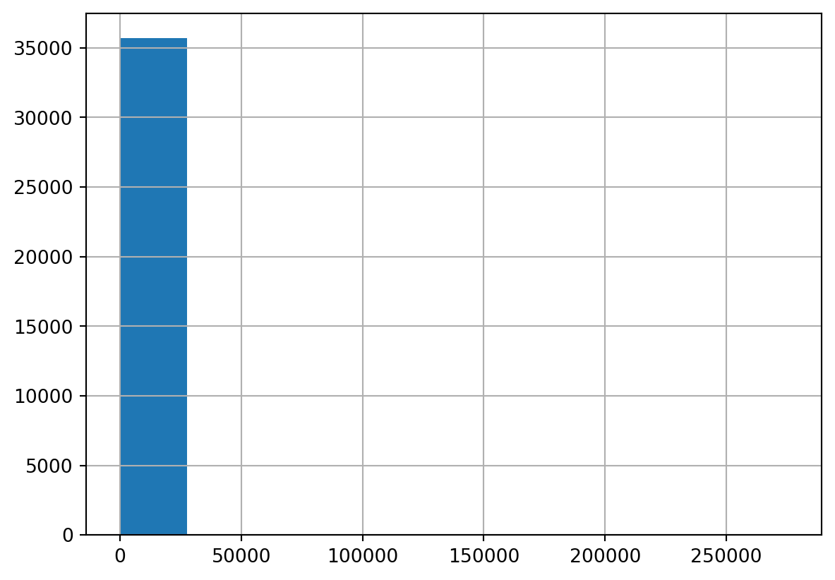
The equivalent code with matplotlib would be:
import matplotlib.pyplot as plt
plt.plot(df.index, df['Déchets'])
By default, the obtained visualization is a series. This is not necessarily what is expected since it only makes sense for time series. As a data scientist working with microdata, you are more often interested in a histogram to get an idea of the data distribution. To do this, simply add the argument kind = 'hist':
df['Déchets'].hist()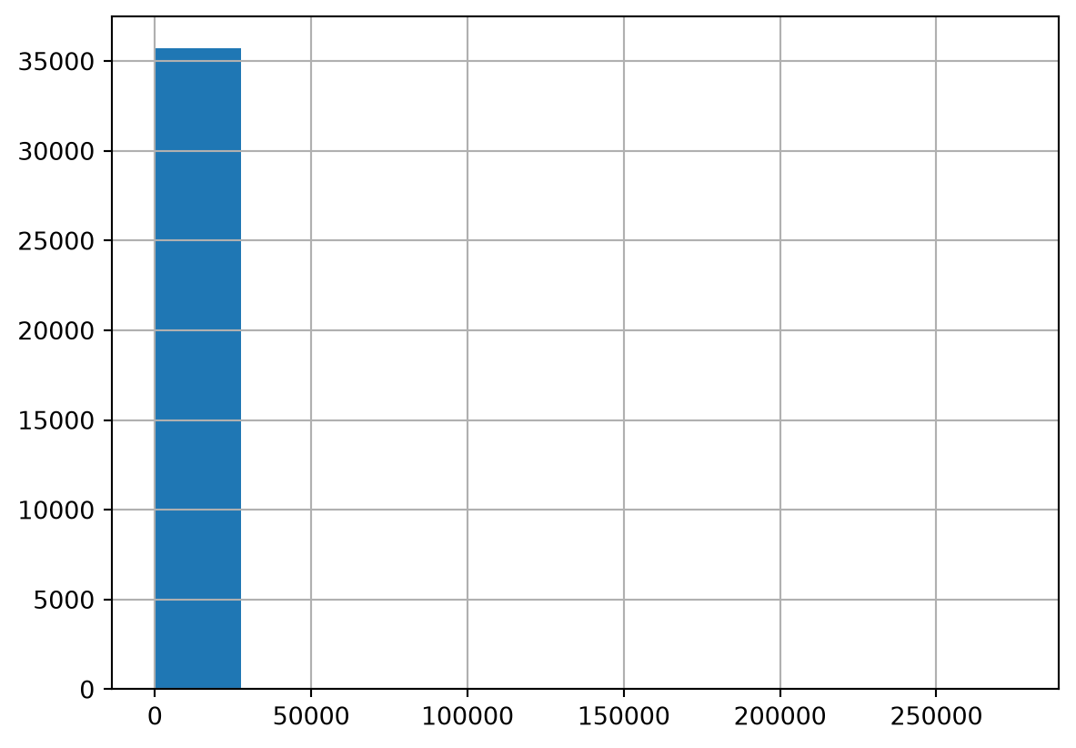
With data that has a non-normalized distribution, which represents many real-world variables, histograms are generally not very informative. The log can be a solution to bring some extreme values to a comparable scale:
df['Déchets'].plot(kind = 'hist', logy = True)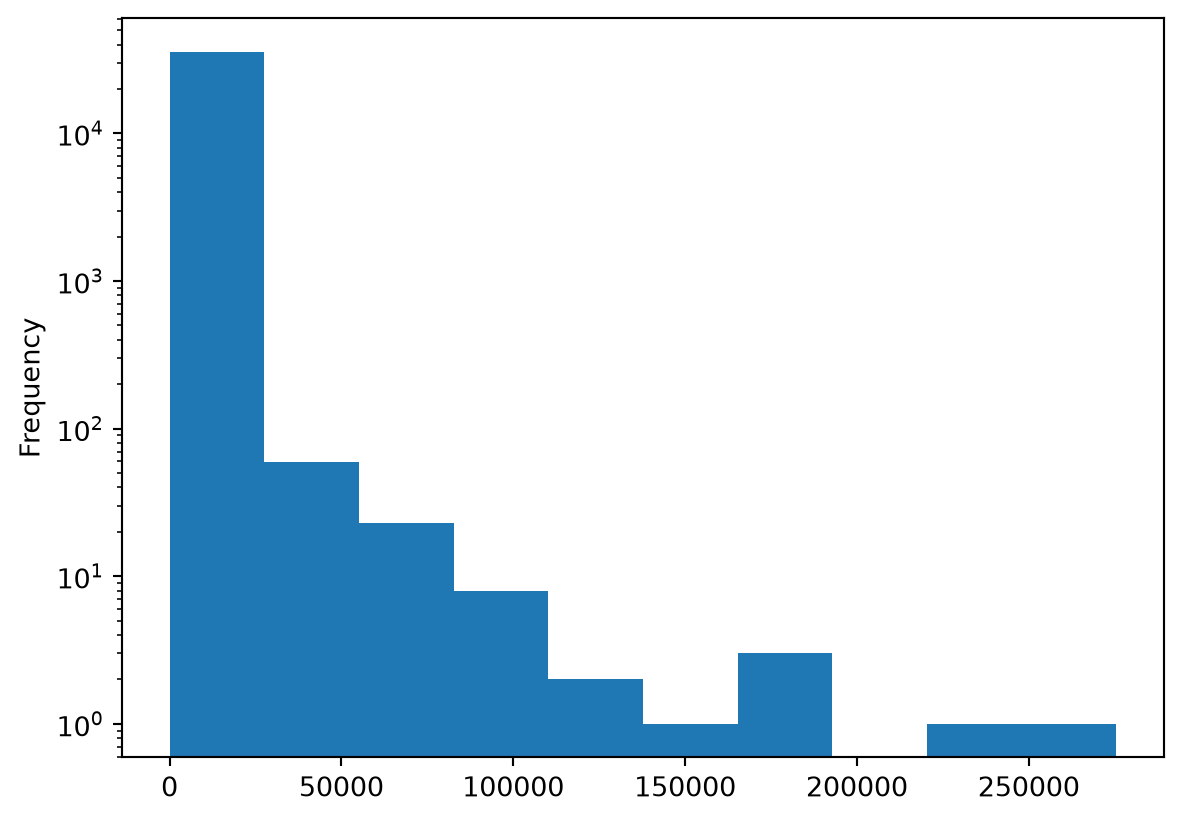
The output is a matplotlib object. Customizing these figures is thus possible (and even desirable because the default matplotlib graphs are quite basic). However, this is a quick method for constructing figures that require work for a finalized visualization. This involves thorough work on the matplotlib object or using a higher-level library for graphical representation (seaborn, plotnine, plotly, etc.).
The part of this course dedicated to data visualization will briefly present these different visualization paradigms. These do not exempt you from using common sense in choosing the graph used to represent a descriptive statistic (see this conference by Eric Mauvière).
9 Synthesis exercise
This exercise synthesizes several steps of data preparation and exploration to better understand the structure of the phenomenon we want to study, namely carbon emissions in France.
It is recommended to start from a clean session (in a notebook, you should do Restart Kernel) to avoid an environment polluted by other objects. You can then run the following code to get the necessary base:
import pandas as pd

emissions = pd.read_csv("https://koumoul.com/s/data-fair/api/v1/datasets/igt-pouvoir-de-rechauffement-global/convert")
emissions.head(2)| INSEE commune | Commune | Agriculture | Autres transports | Autres transports international | CO2 biomasse hors-total | Déchets | Energie | Industrie hors-énergie | Résidentiel | Routier | Tertiaire | |
|---|---|---|---|---|---|---|---|---|---|---|---|---|
| 0 | 01001 | L'ABERGEMENT-CLEMENCIAT | 3711.425991 | NaN | NaN | 432.751835 | 101.430476 | 2.354558 | 6.911213 | 309.358195 | 793.156501 | 367.036172 |
| 1 | 01002 | L'ABERGEMENT-DE-VAREY | 475.330205 | NaN | NaN | 140.741660 | 140.675439 | 2.354558 | 6.911213 | 104.866444 | 348.997893 | 112.934207 |
TipExercise 2: Discovering the Pandas Verbs for Data Manipulation
First, let’s get familiar with operations on columns.
- Create a
DataFrameemissions_copykeeping only the columnsINSEE commune,Commune,Autres transports, andAutres transports international.
Hint for this question
- Since the variable names are not practical, rename them as follows:
INSEE commune\(\to\)code_inseeAutres transports\(\to\)transportsAutres transports international\(\to\)transports_international
Hint for this question
For simplicity, replace missing values (
NA) with 0. Use thefillnamethod to transform missing values into 0.Create the following variables:
dep: the department. This can be created using the first two characters ofcode_inseeby applying thestrmethod;transports_total: the emissions of the transport sector (sum of the two variables).
Hint for this question
- Order the data from the biggest polluter to the smallest, then order the data from the biggest polluter to the smallest by department (from 01 to 95).
Hint for this question
- Keep only the municipalities belonging to departments 13 or 31. Order these municipalities from the biggest polluter to the smallest.
Hint for this question
Return to the initial emission dataset.
Calculate the total emissions by sector. Calculate the share of each sector in total emissions. Convert the volumes to tons before displaying the results.
Calculate the total emissions for each municipality after imputing missing values to 0. Keep the top 100 emitting municipalities. Calculate the share of each sector in this emission. Understand the factors that may explain this ranking.
Help if you are struggling with question 8
Play with the axis parameter when constructing an aggregate statistic.
In question 5, when the communes are ordered exclusively on the basis of the variable transport_total, the result is as follows:
| code_insee | Commune | transports | transports_international | dep | transports_total | |
|---|---|---|---|---|---|---|
| 31108 | 77291 | LE MESNIL-AMELOT | 133834.090767 | 3.303394e+06 | 77 | 3.437228e+06 |
| 31099 | 77282 | MAUREGARD | 133699.072712 | 3.303394e+06 | 77 | 3.437093e+06 |
| 31111 | 77294 | MITRY-MORY | 89815.529858 | 2.202275e+06 | 77 | 2.292090e+06 |
Question 6 gives us this classification:
| code_insee | Commune | transports | transports_international | dep | transports_total | |
|---|---|---|---|---|---|---|
| 4438 | 13096 | SAINTES-MARIES-DE-LA-MER | 271182.758578 | 0.000000 | 13 | 271182.758578 |
| 4397 | 13054 | MARIGNANE | 245375.418650 | 527360.799265 | 13 | 772736.217915 |
| 11684 | 31069 | BLAGNAC | 210157.688544 | 403717.366279 | 31 | 613875.054823 |
In question 7, the resulting table looks like this
| secteur | emissions | emissions (%) | |
|---|---|---|---|
| 2 | transports_total | 28774.0 | 50.0 |
| 1 | transports_international | 22239.0 | 39.0 |
| 0 | transports | 6535.0 | 11.0 |
| INSEE commune | Commune | Agriculture | Autres transports | Autres transports international | CO2 biomasse hors-total | Déchets | Energie | Industrie hors-énergie | Résidentiel | Routier | Tertiaire | |
|---|---|---|---|---|---|---|---|---|---|---|---|---|
| 4382 | 13039 | FOS-SUR-MER | 305.092893 | 1893.383189 | 1.722723e+04 | 50891.367548 | 275500.374439 | 2.296711e+06 | 6.765119e+06 | 9466.388806 | 74631.401993 | 42068.140058 |
| 22671 | 59183 | DUNKERQUE | 811.390947 | 3859.548994 | 3.327586e+05 | 71922.181764 | 23851.780482 | 1.934988e+06 | 5.997333e+06 | 113441.727216 | 94337.865738 | 70245.678455 |
| 4398 | 13056 | MARTIGUES | 855.299300 | 2712.749275 | 3.043476e+04 | 35925.561051 | 44597.426397 | 1.363402e+06 | 2.380185e+06 | 22530.797276 | 84624.862481 | 44394.822725 |
| 30560 | 76476 | PORT-JEROME-SUR-SEINE | 2736.931327 | 121.160849 | 2.086403e+04 | 22846.964780 | 78.941581 | 1.570236e+06 | 2.005643e+06 | 21072.566129 | 9280.824961 | 15270.357772 |
| 31108 | 77291 | LE MESNIL-AMELOT | 782.183307 | 133834.090767 | 3.303394e+06 | 3330.404124 | 111.613197 | 8.240952e+02 | 2.418925e+03 | 1404.400153 | 11712.541682 | 13680.471909 |
| ... | ... | ... | ... | ... | ... | ... | ... | ... | ... | ... | ... | ... |
| 30056 | 74281 | THONON-LES-BAINS | 382.591429 | 145.151526 | 0.000000e+00 | 144503.815623 | 21539.524775 | 2.776024e+03 | 1.942086e+05 | 44545.339492 | 25468.667604 | 19101.562585 |
| 33954 | 86194 | POITIERS | 2090.630127 | 20057.297403 | 2.183418e+04 | 95519.054766 | 13107.640015 | 5.771021e+03 | 1.693938e+04 | 110218.156827 | 91921.787626 | 73121.300634 |
| 1918 | 06019 | BLAUSASC | 194.382622 | 0.000000 | 0.000000e+00 | 978.840592 | 208.084792 | 2.260375e+02 | 4.362880e+05 | 538.816198 | 3949.838612 | 740.022785 |
| 27607 | 68253 | OTTMARSHEIM | 506.238288 | 679.598495 | 3.526748e+01 | 4396.853500 | 237.508651 | 1.172570e+03 | 4.067258e+05 | 3220.875864 | 19317.977050 | 4921.144781 |
| 28643 | 71076 | CHALON-SUR-SAONE | 1344.584721 | 1336.547546 | 6.558180e+01 | 77082.218324 | 570.662275 | 1.016933e+04 | 2.075650e+05 | 77330.230592 | 29020.646500 | 34997.262920 |
100 rows × 12 columns
At the end of question 8, we better understand the factors that can explain high emissions at the municipal level. If we look at the top three emitting municipalities, we can see that they are cities with refineries:
| INSEE commune | Commune | Agriculture | Autres transports | Autres transports international | CO2 biomasse hors-total | Déchets | Energie | Industrie hors-énergie | Résidentiel | ... | Part Autres transports | Part Autres transports international | Part CO2 biomasse hors-total | Part Déchets | Part Energie | Part Industrie hors-énergie | Part Résidentiel | Part Routier | Part Tertiaire | Part total | |
|---|---|---|---|---|---|---|---|---|---|---|---|---|---|---|---|---|---|---|---|---|---|
| 4382 | 13039 | FOS-SUR-MER | 305.092893 | 1893.383189 | 17227.234585 | 50891.367548 | 275500.374439 | 2.296711e+06 | 6.765119e+06 | 9466.388806 | ... | 0.019860 | 0.180696 | 0.533799 | 2.889719 | 24.090160 | 70.959215 | 0.099293 | 0.782807 | 0.441252 | 100.0 |
| 22671 | 59183 | DUNKERQUE | 811.390947 | 3859.548994 | 332758.630269 | 71922.181764 | 23851.780482 | 1.934988e+06 | 5.997333e+06 | 113441.727216 | ... | 0.044652 | 3.849791 | 0.832091 | 0.275949 | 22.386499 | 69.385067 | 1.312444 | 1.091425 | 0.812695 | 100.0 |
| 4398 | 13056 | MARTIGUES | 855.299300 | 2712.749275 | 30434.762405 | 35925.561051 | 44597.426397 | 1.363402e+06 | 2.380185e+06 | 22530.797276 | ... | 0.067655 | 0.759035 | 0.895975 | 1.112249 | 34.002905 | 59.361219 | 0.561912 | 2.110523 | 1.107196 | 100.0 |
3 rows × 24 columns
Thanks to our minimal explorations with Pandas, we see that this dataset provides information about the nature of the French productive fabric and the environmental consequences of certain activities.
References
The site pandas.pydata serves as a reference
The book
Modern Pandasby Tom Augspurger: https://tomaugspurger.github.io/modern-1-intro.html
McKinney, Wes. 2012. Python for Data Analysis: Data Wrangling with Pandas, NumPy, and IPython. " O’Reilly Media, Inc.".
Wickham, Hadley, Mine Çetinkaya-Rundel, and Garrett Grolemund. 2023. R for Data Science. " O’Reilly Media, Inc.".
Informations additionnelles
NotePython environment
This site was built automatically through a Github action using the Quarto
The environment used to obtain the results is reproducible via uv. The pyproject.toml file used to build this environment is available on the linogaliana/python-datascientist repository
pyproject.toml
[project]
name = "python-datascientist"
version = "0.1.0"
description = "Source code for Lino Galiana's Python for data science course"
readme = "README.md"
requires-python = ">=3.13,<3.14"
dependencies = [
    "altair>=6.0.0",
    "cartiflette",
    "contextily==1.6.2",
    "duckdb>=0.10.1",
    "folium>=0.19.6",
    "gdal==3.11.4",
    "graphviz==0.20.3",
    "great-tables>=0.12.0",
    "gt-extras>=0.0.8",
    "ipykernel>=6.29.5",
    "jupyter>=1.1.1",
    "jupyter-cache>=1.0.0",
    "kaleido>=0.2.1",
    "langchain-community>=0.3.27",
    "loguru==0.7.3",
    "markdown>=3.8",
    "nbclient>=0.10.0",
    "nbformat>=5.10.4",
    "nltk>=3.9.1",
    "pandas>=3.0",
    "pip>=25.1.1",
    "plotly>=6.1.2",
    "plotnine>=0.15",
    "polars>=1.8.2",
    "pyarrow>=17.0.0",
    "pynsee>=0.1.8",
    "python-dotenv>=1.0.1",
    "python-frontmatter>=1.1.0",
    "pywaffle>=1.1.1",
    "requests>=2.32.3",
    "scikit-image>=0.24.0",
    "scikit-learn>=1.8.0",
    "scipy>=1.13.0",
    "seaborn>=0.13.2",
    "selenium<4.39.0",
    "spacy>=3.8.4",
    "webdriver-manager>=4.0.2",
    "wordcloud==1.9.3",
]

[tool.uv.sources]
cartiflette = { git = "https://github.com/inseefrlab/cartiflette" }
gdal = [
  { index = "gdal-wheels", marker = "sys_platform == 'linux'" },
  { index = "geospatial_wheels", marker = "sys_platform == 'win32'" },
]

[[tool.uv.index]]
name = "geospatial_wheels"
url = "https://nathanjmcdougall.github.io/geospatial-wheels-index/"
explicit = true

[[tool.uv.index]]
name = "gdal-wheels"
url = "https://gitlab.com/api/v4/projects/61637378/packages/pypi/simple"
explicit = true

[dependency-groups]
dev = [
    "nb-clean>=4.0.1",
]
To use exactly the same environment (version of Python and packages), please refer to the documentation for uv.
NoteFile history
| SHA | Date | Author | Description |
|---|---|---|---|
| 068ae87a | 2026-07-15 21:47:10 | Lino Galiana | Upgrade Pandas 3.0 (#700) |
| 56ad5bc8 | 2026-07-14 21:57:39 | Lino Galiana | Données filosofi plus à jour pour le chapitre Pandas (#699) |
| d555fa72 | 2025-09-24 08:39:27 | lgaliana | warninglang partout |
| 6d37e77a | 2025-09-23 22:58:21 | Lino Galiana | Correction des problèmes du notebook Pandas (#653) |
| 794ce14a | 2025-09-15 16:21:42 | lgaliana | retouche quelques abstracts |
| eeb949c8 | 2025-08-21 17:38:40 | Lino Galiana | Fix a few problems detected by AI agent (#641) |
| 7006f605 | 2025-07-28 14:20:47 | Lino Galiana | Une première PR qui gère plein de bugs détectés par Nicolas (#630) |
| 99ab48b0 | 2025-07-25 18:50:15 | Lino Galiana | Utilisation des callout classiques pour les box notes and co (#629) |
| 94648290 | 2025-07-22 18:57:48 | Lino Galiana | Fix boxes now that it is better supported by jupyter (#628) |
| 91431fa2 | 2025-06-09 17:08:00 | Lino Galiana | Improve homepage hero banner (#612) |
| 388fd975 | 2025-02-28 17:34:09 | Lino Galiana | Colab again and again… (#595) |
| 488780a4 | 2024-09-25 14:32:16 | Lino Galiana | Change badge (#556) |
| 4404ec10 | 2024-09-21 18:28:42 | lgaliana | Back to eval true |
| 72d44dd6 | 2024-09-21 12:50:38 | lgaliana | Force build for pandas chapters |
| f4367f78 | 2024-08-08 11:44:37 | Lino Galiana | Traduction chapitre suite Pandas avec un profile (#534) |
| 580cba77 | 2024-08-07 18:59:35 | Lino Galiana | Multilingual version as quarto profile (#533) |
| 72f42bb7 | 2024-07-25 19:06:38 | Lino Galiana | Language message on notebooks (#529) |
| 195dc9e9 | 2024-07-25 11:59:19 | linogaliana | Switch language button |
| 6ca4c1c7 | 2024-07-08 17:24:11 | Lino Galiana | Traduction du premier chapitre Pandas (#520) |
| ce13b918 | 2024-07-07 21:14:21 | Lino Galiana | Lua filter for callouts (both html AND ipynb output format) !! 🎉 (#511) |
| a987feaa | 2024-06-23 18:43:06 | Lino Galiana | Fix broken links (#506) |
| 91bfa525 | 2024-05-27 15:01:32 | Lino Galiana | Restructuration partie geopandas (#500) |
| e0d615e3 | 2024-05-03 11:15:29 | Lino Galiana | Restructure la partie Pandas (#497) |
Footnotes
The equivalent ecosystem in
R, thetidyverse, developed by Posit, is of more recent design thanPandas. Its philosophy could thus draw inspiration fromPandaswhile addressing some limitations of thePandassyntax. Since both syntaxes are an implementation inPythonorRof theSQLphilosophy, it is natural that they resemble each other and that it is pertinent for data scientists to know both languages.↩︎Actually, it is not the carbon footprint but the national inventory since the database corresponds to a production view, not consumption. Emissions made in one municipality to satisfy the consumption of another will be attributed to the former where the carbon footprint concept would attribute it to the latter. Moreover, the emissions presented here do not include those produced by goods made abroad. This exercise is not about constructing a reliable statistic but rather understanding the logic of data merging to construct descriptive statistics.↩︎
The original goal of
Pandasis to provide a high-level library for more abstract low-level layers, such asNumpyarrays.Pandasis gradually changing these low-level layers to favorArrowoverNumpywithout destabilizing the high-level commands familiar toPandasusers. This shift is due to the fact thatArrow, a low-level computation library, is more powerful and flexible thanNumpy. For example,Numpyoffers limited textual types, whereasArrowprovides greater freedom.↩︎Due to a lack of imagination, we are often tempted to call our main dataframe
dfordata. This is often a bad idea because the name is not very informative when you read the code a few weeks later. Self-documenting code, an approach that consists of having code that is self-explanatory, is a good practice, and it is recommended to give a simple yet effective name to know the nature of the dataset in question.↩︎
Citation
BibTeX citation:
@book{galiana2025,
  author = {Galiana, Lino},
  title = {Python Pour La Data Science},
  date = {2025},
  url = {https://pythonds.linogaliana.fr/},
  doi = {10.5281/zenodo.8229676},
  langid = {en}
}
For attribution, please cite this work as:
Galiana, Lino. 2025. Python Pour La Data Science. https://doi.org/10.5281/zenodo.8229676.