Python pour la data science

Lino Galiana

doi:10.5281/zenodo.8229676

If you want to try the examples in this tutorial:

In the previous chapters, we explored how to retrieve and harmonize data from various source: CSV files, APIs, web scraping, and more. However, no overview of data access methods would be complete without mentioning a relatively recent addition to the data ecosystem: the Parquet data format.

Thanks to its technical advantages - specifically designed for analytical workloads - and its seamless integration with Python, Parquet is becoming increasingly essential. It has, in fact, become a key component of modern cloud infrastructures, which have emerged since the mid-2010s as the standard environment for data science workflows.¹

Objectives

Understand the challenges involved in storing and processing different types of data formats
Distinguish between file-based storage and database systems
Discover Parquet format and its advantages over flat files and proprietary formats
Learn how to work with Parquet data using Arrow and DuckDB
Explore the implications of cloud-based storage and how Python can adapt to modern data infrastructures

1 Contextual Elements

1.1 Principles of Data Storage

Before exploring the advantages of the Parquet format, it is helpful to briefly review how data is stored and made accessible to a processing language like Python².

Two main approaches coexist: file-based storage and relational database storage. The key distinction between these paradigms lies in how access to data is structured and managed.

1.2 File-Based Storage

1.2.1 Flat Files

In a flat file, data is organized in a linear fashion, with values typically separated by a delimiter such as a comma, semicolon, or tab. Here’s a simple example using a .csv file:

nom ; profession 
Astérix ; 
Obélix ; Tailleur de menhir ;
Assurancetourix ; Barde

Python can easily structure this information:

	nom	profession
0	Astérix
1	Obélix	Tailleur de menhir
2	Assurancetourix	Barde

StringIO permet de traiter la chaîne de caractère comme le contenu d’un fichier.

These are referred to as flat files because all the records related to a given observation are stored sequentially, without any hierarchical structure.

1.2.2 Hierarchical files

Other formats, such as JSON, structure data in a hierarchical way:

[
  {
    "nom": "Astérix"
  },
  {
    "nom": "Obélix",
    "profession": "Tailleur de menhir"
  },
  {
    "nom": "Assurancetourix",
    "profession": "Barde"
  }
]

In such cases, when information is missing - as in the line for “Astérix” - you don’t see two delimiters side by side. Instead, the missing data is simply left out.

Caution

The difference between a .csv file and a JSON file lies not only in their format but also in their underlying logic of data storage.

JSON is a non-tabular format that offers greater flexibility: it allows the structure of the data to evolve over time without requiring previous entries to be modified or recompiled. This makes it particularly well-suited for dynamic data collection environments, such as APIs.

For instance, a website that begins collecting a new piece of information doesn’t need to retroactively update all prior records. It can simply add the new field to the relevant entries—omitting it from others where the information wasn’t collected.

It is then up to the query tool—such as Python or another platform—to reconcile and link data across these differing structures.

This flexible approach underpins many NoSQL databases (like ElasticSearch), which play a central role in the big data ecosystem.

1.2.3 Data split across multiple files

It is common for a single observation to be distributed across multiple files in different formats. In geomatics, for example, geographic boundaries are often stored separately from the data that gives them context:

In some cases, everything is bundled into a single file that contains both the geographic shapes and the associated attribute values. This is the approach used by formats like GeoJSON;
In other cases, the data is split across several files, and reading the full information - geographic shapes, data for each zone, projection system, etc. - requires combining them. This is the case with the Shapefile format.

When data is distributed across multiple files, this is up to the processing tool (e.g., Python) to perform the necessary joins and link the information together.

1.2.4 The role of the file system

The file system enables the computer to locate files physically on the disk. It plays a central role in file management, handling file naming, folder hierarchy, and access permissions.

1.3 Storing Data in a Database

The logic behind databases differs fundamentally and is more systematic in nature. A relational database is managed by a Database Management System (DBMS), which provides capabilities for:

storing coherent datasets;
performing updates (insertions, deletions, modifications);
controlling access (user permissions, query types, etc.).

Data is organized into tables connected by relationships, often structured according to a star schema:

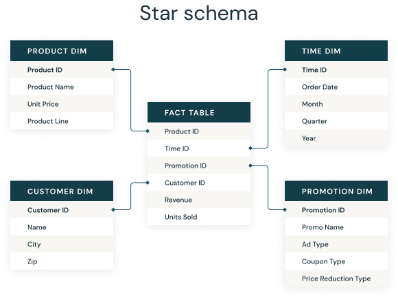
The software managing the database links these tables together using SQL queries. One of the most powerful and widely used systems for this purpose is PostgreSQL.

Python can interact with databases by issuing SQL queries. Historically, packages such as sqlalchemy and psycopg2 have been standard tools for communicating with PostgreSQL databases, enabling both reading and updating operations. More recently, DuckDB has emerged as a lightweight and user-friendly alternative for querying relational data, and it will be discussed again in the context of the Parquet format.

Why File-Based Storage is gaining popularity

The increasing popularity of file-based storage in the data science ecosystem is due to a number of technical and practical advantages that make it well-suited for modern analytical workflows.

Files are generally more lightweight and easier to manage than databases. They do not require the installation or maintenance of specialized software; a basic file system, available on every operating system, is sufficient for accessing them.

Reading a file in Python simply involves using a library such as Pandas. In contrast, interacting with a database typically requires:

installing and configuring a DBMS (e.g., PostgreSQL, MySQL);
managing network connections;
relying on libraries such as sqlalchemy or psycopg2.

This additional complexity makes file-based workflows more flexible and faster for exploratory tasks.

However, this simplicity comes with limitations. File-based systems generally lack fine-grained access control. For instance, preventing a user from modifying or deleting a file is difficult without duplicating it and working from a copy. This represents a constraint in multi-user environments, although cloud-based storage solutions — particularly S3 technology, which will be addressed later — offer effective remedies.

The primary reason why files are often preferred over DBMSs lies in the nature of the operations being performed. Relational databases are particularly well-suited for contexts involving frequent updates or complex operations on structured data — a typical application logic, in which data is continuously evolving (through insertions, updates, or deletions).

By contrast, in analytical contexts, the focus is on reading and temporarily manipulating data without altering the original source. The objective is to query, aggregate, and filter — not to persist changes. In such scenarios, files (especially when stored in optimized formats like Parquet) are ideal: they offer fast read times, high portability, and eliminate the overhead associated with running a full database engine.

2 The `Parquet` format

The CSV format has long been popular for its simplicity:

It is human-readable (any text editor can open it);
It relies on a simple tabular structure, well-suited for many analytical situations;
It is universal and interoperable, as it is not tied to any specific software.

However, this simplicity comes at a cost. Several limitations of the CSV format have led to the emergence of more efficient formats for data analysis, such as Parquet.

2.1 Limitations of the `CSV` format

CSV is a heavy format:

It is not compressed, increasing its disk size;
All data is stored as raw text. Data type optimization (integer, float, string, etc.) is deferred to the importing library (like Pandas), which must scan the data at load time—slowing down performance and increasing error risk.

CSV is row-oriented:

To access a specific column, every row must be read, and the relevant column extracted;
This model performs poorly when only a subset of columns is needed—a common case in data science.

CSV is expensive to modify:

Adding a column or inserting intermediate data requires rewriting the entire file. For example, adding a hair column would mean generating a new version of the file:
```
name ; hair ; profession
Asterix ; blond ; 
Obelix ; redhead ; Menhir sculptor
Assurancetourix ; blond ; Bard
```

About proprietary formats

Most data science tools offer their own serialization formats:

.pickle for Python,
.rda or .RData for R,
.dta for Stata,
.sas7bdat for SAS.

However, these formats are proprietary or tightly coupled to one language, which raises interoperability issues. For example, Python cannot natively read .sas7bdat. Even when third-party libraries exist, the lack of official documentation makes support unreliable.

In this regard, despite its limitations, .csv remains popular for its universality. But the Parquet format offers both this portability and significantly better performance.

2.2 The Rise of the `Parquet` Format

To address these limitations, the Parquet format—developed as an Apache open-source project offers a radically different approach.

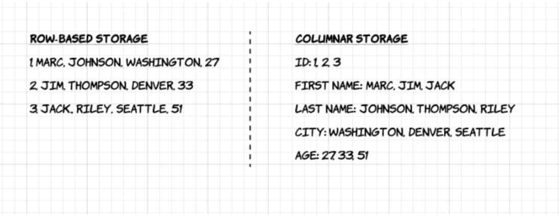
Its key characteristic: it is column-oriented. Unlike CSVs, data for each column is stored separately. This allows:

loading only the columns relevant for analysis;
more efficient data compression;
significantly faster selective queries.

Here’s a diagram from the Upsolver blog illustrating the difference between row-based and columnar storage:

In our example, you could read the profession column without parsing names, making access faster (ignore the pyarrow.Table element—we’ll return to it later):

pyarrow.Table
nom : string
profession: string
----
nom : [["Astérix ","Obélix ","Assurancetourix "]]
profession: [["","Tailleur de menhir","Barde"]]

Thanks to the column-oriented structure, it is possible to read only a single variable (such as profession) without having to scan every row in the file.

path
└── to
    └── table
        ├── gender=male
        │   ├── country=US
        │   │   └── data.parquet
        │   ├── country=CN
        │   │   └── data.parquet
        └── gender=female
            ├── country=US
            │   └── data.parquet
            ├── country=CN
            │   └── data.parquet

When read, the entire dataset is reconstructed into a tabular format:

root
|-- name: string (nullable = true)
|-- age: long (nullable = true)
|-- gender: string (nullable = true)
|-- country: string (nullable = true)

2.3 A format designed for analysis — not just big data

As emphasized in the Upsolver blog:

Complex data such as logs and event streams would need to be represented as a table with hundreds or thousands of columns, and many millions of rows. Storing this table in a row-based format such as CSV would mean:

Queries will take longer to run since more data needs to be scanned…

Storage will be more costly since CSVs are not compressed as efficiently as Parquet

However, the Parquet format is not limited to big data architectures. Its advantages are accessible to anyone who produces or works with datasets, regardless of scale:

significantly reduced file sizes;
fast, reliable, and memory-efficient data import.

The translation of this chapter is still in progress. The remaining sections will be available soon.

2.4 Reading a `Parquet` file in `Python`: example

There are many libraries that integrate well with the Parquet format, but the two most important to know are PyArrow and DuckDB. These libraries were previously mentioned as alternatives to Pandas for handling larger-than-memory datasets. They are often used to perform heavy initial operations before converting the results into a lightweight pd.DataFrame for further analysis.

The PyArrow library enables efficient reading and writing of Parquet files by taking advantage of their columnar structure³. It operates on a pyarrow.Table object, which—after processing—can be converted to a Pandas DataFrame to leverage the broader capabilities of the Pandas ecosystem.

The DuckDB library allows you to query Parquet files directly using SQL, without loading the entire file into memory. In essence, it brings the database philosophy (structured queries via SQL) to file-based storage. The results of such queries can also be converted into a Pandas DataFrame, combining the convenience of Pandas with the efficiency of an embedded SQL engine.

A lesser-known but valuable feature of DuckDB is its ability to perform SQL queries directly on a Pandas DataFrame. This can be especially useful when Pandas syntax becomes verbose or cumbersome—for example, when computing a new column based on grouped statistics, where SQL expressions can be more concise and readable.

Tip

Using pa for pyarrow and pq for pyarrow.parquet is a widely adopted convention, much like using pd for pandas.

To demonstrate these features, we will use a dataset derived from the synthetic census data published by Insee, the French national statistics agency.

import requests
import pyarrow.parquet as pq

# Example Parquet
url = "https://minio.lab.sspcloud.fr/projet-formation/bonnes-pratiques/data/RPindividus/REGION=93/part-0.parquet"

# Télécharger le fichier et l'enregistrer en local
with open("example.parquet", "wb") as f:
    response = requests.get(url)
    f.write(response.content)

Arrow
DuckDB

To fully benefit from the optimizations provided by the Parquet format, it is recommended to use pyarrow.dataset. This approach makes it possible to take full advantage of the performance gains offered by the combination of Parquet and Arrow, which are not always accessible when reading Parquet files using other methods available in the Arrow ecosystem (as will be explored in upcoming exercises).

import pyarrow.dataset as ds

dataset = ds.dataset(
  "example.parquet"
).scanner(columns = ["AGED", "IPONDI", "DEPT"])
table = dataset.to_table()
table

pyarrow.Table
AGED: int32
IPONDI: double
DEPT: dictionary<values=string, indices=int32, ordered=0>
----
AGED: [[9,12,40,70,52,...,29,66,72,75,77],[46,76,46,32,2,...,7,5,37,29,4],...,[67,37,45,56,75,...,64,37,47,20,18],[16,25,51,6,11,...,93,90,92,21,65]]
IPONDI: [[2.73018871840726,2.73018871840726,2.73018871840726,0.954760150327854,3.75907197064638,...,3.27143319621654,4.83980378599556,4.83980378599556,4.83980378599556,4.83980378599556],[3.02627578376137,3.01215358930406,3.01215358930406,2.93136309038958,2.93136309038958,...,2.96848755763453,2.96848755763453,3.25812879950072,3.25812879950072,1.12514509319438],...,[2.57931132917563,2.85579410739065,0.845993555838931,2.50296716736141,3.70786113613679,...,3.08375347880892,2.88038807573222,3.22776230929947,3.22776230929947,3.22776230929947],[3.22776230929947,3.22776230929947,3.22776230929947,3.29380242174036,3.29380242174036,...,5.00000768518755,5.00000768518755,5.00000768518755,5.00000768518755,1.00000153703751]]
DEPT: [  -- dictionary:
["01","02","03","04","05",...,"95","971","972","973","974"]  -- indices:
[5,5,5,5,5,...,5,5,5,5,5],  -- dictionary:
["01","02","03","04","05",...,"95","971","972","973","974"]  -- indices:
[5,5,5,5,5,...,5,5,5,5,5],...,  -- dictionary:
["01","02","03","04","05",...,"95","971","972","973","974"]  -- indices:
[84,84,84,84,84,...,84,84,84,84,84],  -- dictionary:
["01","02","03","04","05",...,"95","971","972","973","974"]  -- indices:
[84,84,84,84,84,...,84,84,84,84,84]]

To import and process these data, one can either keep the data in pyarrow.Table format or convert it into a pandas.DataFrame. The second option is slower but has the advantage of enabling all the manipulations offered by the pandas ecosystem, which is generally more familiar than that of Arrow.

import duckdb
duckdb.sql("""
FROM read_parquet('example.parquet')
SELECT AGED, IPONDI, DEPT
""")

┌───────┬───────────────────┬─────────┐
│ AGED  │      IPONDI       │  DEPT   │
│ int32 │      double       │ varchar │
├───────┼───────────────────┼─────────┤
│     9 │  2.73018871840726 │ 06      │
│    12 │  2.73018871840726 │ 06      │
│    40 │  2.73018871840726 │ 06      │
│    70 │ 0.954760150327854 │ 06      │
│    52 │  3.75907197064638 │ 06      │
│    82 │  3.21622922493506 │ 06      │
│     6 │  3.44170061276923 │ 06      │
│    12 │  3.44170061276923 │ 06      │
│    15 │  3.44170061276923 │ 06      │
│    43 │  3.44170061276923 │ 06      │
│     · │          ·        │ ·       │
│     · │          ·        │ ·       │
│     · │          ·        │ ·       │
│    68 │  2.73018871840726 │ 06      │
│    35 │  3.46310256220757 │ 06      │
│     2 │  3.46310256220757 │ 06      │
│    37 │  3.46310256220757 │ 06      │
│    84 │  3.69787960424482 │ 06      │
│    81 │   4.7717265388427 │ 06      │
│    81 │   4.7717265388427 │ 06      │
│    51 │  3.60566450823737 │ 06      │
│    25 │  3.60566450823737 │ 06      │
│    13 │  3.60566450823737 │ 06      │
├───────┴───────────────────┴─────────┤
│    ? rows (>9999 rows, 20 shown)    │
└─────────────────────────────────────┘

2.5 Exercises to Learn More

The following is a series of exercises adapted from the production deployment of data science projects course, which Romain Avouac and I teach in the final year of the engineering program at ENSAE.

These exercises progressively illustrate some of the key concepts discussed above, while also emphasizing best practices for working with large-scale data. Solutions to all exercises are available on the corresponding course page.

In this practical section, we will explore how to use the Parquet format as efficiently as possible. To compare different data formats and access strategies, we will measure and compare the execution time and memory usage of a standard query. We will begin with a lightweight example that compares the performance of reading data in CSV versus Parquet format.

To do so, we will first retrieve a dataset in Parquet format. We suggest using the detailed and anonymized French population census data, which contains approximately 20 million rows and 80 columns. The code to download and access this dataset is provided below.

Program to retrieve exercise dataset

import pyarrow.parquet as pq
import pyarrow as pa
import os

# Définir le fichier de destination
filename_table_individu = "data/RPindividus.parquet"

# Copier le fichier depuis le stockage distant (remplacer par une méthode adaptée si nécessaire)
1os.system("mc cp s3/projet-formation/bonnes-pratiques/data/RPindividus.parquet data/RPindividus.parquet")

# Charger le fichier Parquet
table = pq.read_table(filename_table_individu)
df = table.to_pandas()

# Filtrer les données pour REGION == "24"
df_filtered = df.loc[df["REGION"] == "24"]

# Sauvegarder en CSV
df_filtered.to_csv("data/RPindividus_24.csv", index=False)

# Sauvegarder en Parquet
pq.write_table(pa.Table.from_pandas(df_filtered), "data/RPindividus_24.parquet")

1: This line of code uses the Minio Client utility available on the SSPCloud. If you’re not on this infrastructure, please refer to the dedicated box.

If you are not on SSPCloud

You will need to replace the line

os.system("mc cp s3/projet-formation/bonnes-pratiques/data/RPindividus.parquet data/RPindividus.parquet")

which uses the mc command-line tool, with code that downloads this data from the URL https://projet-formation.minio.lab.sspcloud.fr/bonnes-pratiques/data/RPindividus.parquet.

There are many ways to do this. For instance, you can use plain Python with requests. If you have curl installed, you can use it as well. Via Python, this would translate to the command: os.system("curl -o data/RPindividus.parquet https://projet-formation/bonnes-pratiques/data/RPindividus.parquet").

These exercises will make use of Python decorators - functions that modify or extend the behavior of other functions. In our case, we will define a function that performs a series of operations, and then apply a decorator to it that tracks both memory usage and execution time.

Part 1: From CSV to Parquet

Create a notebook named benchmark_parquet.ipynb to perform various performance comparisons throughout the application.
Define a custom decorator that will be used to benchmark the Python code by measuring execution time and memory usage.

Click to expand and view the code for the performance-measuring decorator.

::: {#f81bcb8f .cell execution_count=11} ``` {.python .cell-code} import time from memory_profiler import memory_usage from functools import wraps import warnings

def convert_size(size_bytes):
if size_bytes == 0:
    return "0B"
size_name = ("B", "KB", "MB", "GB", "TB", "PB", "EB", "ZB", "YB")
i = int(math.floor(math.log(size_bytes, 1024)))
p = math.pow(1024, i)
s = round(size_bytes / p, 2)
return "%s %s" % (s, size_name[i])

# Decorator to measure execution time and memory usage
def measure_performance(func, return_output=False):
    @wraps(func)
    def wrapper(return_output=False, *args, **kwargs):
        warnings.filterwarnings("ignore")
        start_time = time.time()
        mem_usage = memory_usage((func, args, kwargs), interval=0.1)
        end_time = time.time()
        warnings.filterwarnings("always")

        exec_time = end_time - start_time
        peak_mem = max(mem_usage)  # Peak memory usage
        exec_time_formatted = f"\033[92m{exec_time:.4f} sec\033[0m"
        peak_mem_formatted = f"\033[92m{convert_size(1024*peak_mem)}\033[0m"

        print(f"{func.__name__} - Execution Time: {exec_time_formatted} | Peak Memory Usage: {peak_mem_formatted}")
        if return_output is True:
            return func(*args, **kwargs)

    return wrapper

:::


</details>

* Reuse this code to wrap the logic for constructing the age pyramid into a function named `process_csv_appli1`.

<details>

<summary>
Click to expand and view the code used to measure the performance of reading CSV files.
</summary>


::: {#96a043fa .cell execution_count=12}
``` {.python .cell-code}
# Apply the decorator to functions
@measure_performance
def process_csv_appli1(*args, **kwargs):
    df = pd.read_csv("data/RPindividus_24.csv")
    return (
        df.loc[df["DEPT"] == 36]
        .groupby(["AGED", "DEPT"])["IPONDI"]
        .sum().reset_index()
        .rename(columns={"IPONDI": "n_indiv"})
    )

:::

Run process_csv_appli1() and process_csv_appli1(return_output=True) to observe performance and optionally return the processed data.
Using the same approach, define a new function named process_parquet_appli1, this time based on the data/RPindividus_24.parquet file, and load it using Pandas’ read_parquet function.
Compare the performance (execution time and memory usage) of the two methods using the benchmarking decorator.

Full correction

import math
import pandas as pd
import time
from memory_profiler import memory_usage
from functools import wraps
import warnings

def convert_size(size_bytes):
   if size_bytes == 0:
       return "0B"
   size_name = ("B", "KB", "MB", "GB", "TB", "PB", "EB", "ZB", "YB")
   i = int(math.floor(math.log(size_bytes, 1024)))
   p = math.pow(1024, i)
   s = round(size_bytes / p, 2)
   return "%s %s" % (s, size_name[i])

# Decorator to measure execution time and memory usage
def measure_performance(func, return_output=False):
    @wraps(func)
    def wrapper(return_output=False, *args, **kwargs):
        warnings.filterwarnings("ignore")
        start_time = time.time()
        mem_usage = memory_usage((func, args, kwargs), interval=0.1)
        end_time = time.time()
        warnings.filterwarnings("always")

        exec_time = end_time - start_time
        peak_mem = max(mem_usage)  # Peak memory usage
        exec_time_formatted = f"\033[92m{exec_time:.4f} sec\033[0m"
        peak_mem_formatted = f"\033[92m{convert_size(1024*peak_mem)}\033[0m"

        print(f"{func.__name__} - Execution Time: {exec_time_formatted} | Peak Memory Usage: {peak_mem_formatted}")
        if return_output is True:
            return func(*args, **kwargs)

    return wrapper

# Apply the decorator to functions
@measure_performance
def process_csv(*args, **kwargs):
    df = pd.read_csv("data/RPindividus_24.csv")
    return (
        df.loc[df["DEPT"] == 36]
        .groupby(["AGED", "DEPT"])["IPONDI"]
        .sum().reset_index()
        .rename(columns={"IPONDI": "n_indiv"})
    )

@measure_performance
def process_parquet(*args, **kwargs):
    df = pd.read_parquet("data/RPindividus_24.parquet")
    return (
        df.loc[df["DEPT"] == "36"]
        .groupby(["AGED", "DEPT"])["IPONDI"]
        .sum().reset_index()
        .rename(columns={"IPONDI": "n_indiv"})
    )

process_csv()
process_parquet()

❓️ What seems to be the limitation of the read_parquet function?

Although we already observe a significant speed improvement during file reading, we are not fully leveraging the optimizations provided by the Parquet format. This is because the data is immediately loaded into a Pandas DataFrame, where transformations are applied afterward.

As a result, we miss out on one of Parquet’s core performance features: predicate pushdown. This optimization allows filters to be applied as early as possible—at the file scan level—so that only the relevant columns and rows are read into memory. By bypassing this mechanism, we lose much of what makes Parquet so efficient in analytical workflows.

Part 2: Leveraging Lazy Evaluation and the Optimizations of Arrow or DuckDB

In the previous section, we observed a significant improvement in read times when switching from CSV to Parquet. However, memory usage remained high, even though only a small portion of the data was actually used.

In this section, we will explore how to take advantage of lazy evaluation and execution plan optimizations offered by Arrow to fully unlock the performance benefits of the Parquet format.

Open the file data/RPindividus_24.parquet using pyarrow.dataset. Check the class of the resulting object.
Run the code below to read a sample of the data:

(
    dataset.scanner()
    .head(5)
    .to_pandas()
)

Can you identify the difference compared to the previous approach? Consult the documentation for the to_table method—do you understand what it does and why it matters?

Create a function summarize_parquet_arrow (and a corresponding summarize_parquet_duckdb) that imports the data using pyarrow.dataset (or DuckDB) and performs the required aggregation.
Use the benchmarking decorator to compare the performance (execution time and memory usage) of the three approaches: reading and processing Parquet data using Pandas, PyArrow, and DuckDB.

Correction

Code complet de l’application

import duckdb
import pyarrow.dataset as ds

@measure_performance
def summarize_parquet_duckdb(*args, **kwargs):
    con = duckdb.connect(":memory:")
    query = """
    FROM read_parquet('data/RPindividus_24.parquet')
    SELECT AGED, DEPT, SUM(IPONDI) AS n_indiv
    GROUP BY AGED, DEPT
    """

    return (con.sql(query).to_df())

@measure_performance
def summarize_parquet_arrow(*args, **kwargs):

    dataset = ds.dataset("data/RPindividus_24.parquet", format="parquet")
    table = dataset.to_table()
    grouped_table = (
        table
        .group_by(["AGED", "DEPT"])
        .aggregate([("IPONDI", "sum")])
        .rename_columns(["AGED", "DEPT", "n_indiv"])
        .to_pandas()
    )

    return (
        grouped_table
    )

process_parquet()
summarize_parquet_duckdb()
summarize_parquet_arrow()

With lazy evaluation, the process unfolds in several stages:

Arrow or DuckDB receives a set of instructions, builds an execution plan, optimizes it, and then executes the query;
Only the final result of this pipeline is returned to Python, rather than the entire dataset.

Part 3a: What Happens When We Filter Rows?

Let us now add a row-level filtering step to our queries:

With DuckDB, modify the SQL query to include a WHERE clause:
WHERE DEPT IN ('18', '28', '36')
With Arrow, update the to_table call as follows:
dataset.to_table(filter=pc.field("DEPT").isin(['18', '28', '36']))

Correction

import pyarrow.dataset as ds
import pyarrow.compute as pc
import duckdb

@measure_performance
def summarize_filter_parquet_arrow(*args, **kwargs):

    dataset = ds.dataset("data/RPindividus.parquet", format="parquet")
    table = dataset.to_table(filter=pc.field("DEPT").isin(['18', '28', '36']))
    grouped_table = (
        table
        .group_by(["AGED", "DEPT"])
        .aggregate([("IPONDI", "sum")])
        .rename_columns(["AGED", "DEPT", "n_indiv"])
        .to_pandas()
    )

    return (
        grouped_table
    )

@measure_performance
def summarize_filter_parquet_duckdb(*args, **kwargs):
    con = duckdb.connect(":memory:")
    query = """
    FROM read_parquet('data/RPindividus_24.parquet')
    SELECT AGED, DEPT, SUM(IPONDI) AS n_indiv
    WHERE DEPT IN ('11','31','34')
    GROUP BY AGED, DEPT
    """

    return (con.sql(query).to_df())

summarize_filter_parquet_arrow()
summarize_filter_parquet_duckdb()

❓️ Why do row filters not improve performance (and sometimes even slow things down), unlike column filters?

This is because data is not stored in row blocks the way it is in column blocks. As a result, filtering rows does not allow the system to skip over large sections of the file as efficiently.

Fortunately, there is a solution: partitioning.

Part 3: Partitioned Parquet

Lazy evaluation and the optimizations available through Arrow already provide significant performance improvements. But we can go even further. When you know in advance that your queries will frequently filter data based on a specific variable, it is highly advantageous to partition the Parquet file using that variable.

Review the documentation for pyarrow.parquet.write_to_dataset to understand how to define a partitioning key when writing a Parquet file. Several approaches are available.
Import the full individuals table from the census using pyarrow.dataset.dataset("data/RPindividus.parquet"), and export it as a partitioned dataset to "data/RPindividus_partitionne.parquet", using both REGION and DEPT as partitioning keys.
Explore the resulting directory structure to examine how partitioning was applied—each partition key should create a subfolder representing a unique value.
Update your data loading, filtering, and aggregation functions (using either Arrow or DuckDB) to operate on the partitioned Parquet file. Then compare the performance with the non-partitioned version.

Correction de la question 2 (écriture du Parquet partitionné)

import pyarrow.parquet as pq
dataset = ds.dataset(
    "data/RPindividus.parquet", format="parquet"
).to_table()

pq.write_to_dataset(
    dataset,
    root_path="data/RPindividus_partitionne",
    partition_cols=["REGION", "DEPT"]
)

Correction de la question 4 (lecture du Parquet partitionné)

import pyarrow.dataset as ds
import pyarrow.compute as pc
import duckdb

@measure_performance
def summarize_filter_parquet_partitioned_arrow(*args, **kwargs):

    dataset = ds.dataset("data/RPindividus_partitionne/", partitioning="hive")
    table = dataset.to_table(filter=pc.field("DEPT").isin(['18', '28', '36']))

    grouped_table = (
        table
        .group_by(["AGED", "DEPT"])
        .aggregate([("IPONDI", "sum")])
        .rename_columns(["AGED", "DEPT", "n_indiv"])
        .to_pandas()
    )

    return (
        grouped_table
    )

@measure_performance
def summarize_filter_parquet_complete_arrow(*args, **kwargs):

    dataset = ds.dataset("data/RPindividus.parquet")
    table = dataset.to_table(filter=pc.field("DEPT").isin(['18', '28', '36']))

    grouped_table = (
        table
        .group_by(["AGED", "DEPT"])
        .aggregate([("IPONDI", "sum")])
        .rename_columns(["AGED", "DEPT", "n_indiv"])
        .to_pandas()
    )

    return (
        grouped_table
    )


@measure_performance
def summarize_filter_parquet_complete_duckdb(*args, **kwargs):
    con = duckdb.connect(":memory:")
    query = """
    FROM read_parquet('data/RPindividus.parquet')
    SELECT AGED, DEPT, SUM(IPONDI) AS n_indiv
    WHERE DEPT IN ('11','31','34')
    GROUP BY AGED, DEPT
    """

    return (con.sql(query).to_df())


@measure_performance
def summarize_filter_parquet_partitioned_duckdb(*args, **kwargs):
    con = duckdb.connect(":memory:")
    query = """
    FROM read_parquet('data/RPindividus_partitionne/**/*.parquet', hive_partitioning = True)
    SELECT AGED, DEPT, SUM(IPONDI) AS n_indiv
    WHERE DEPT IN ('11','31','34')
    GROUP BY AGED, DEPT
    """

    return (con.sql(query).to_df())


summarize_filter_parquet_complete_arrow()
summarize_filter_parquet_partitioned_arrow()
summarize_filter_parquet_complete_duckdb()
summarize_filter_parquet_partitioned_duckdb()

❓️ When delivering data in Parquet format, how should you choose the partitioning key(s)? What limitations should you keep in mind?

3 Data in the Cloud

Cloud storage, in the context of data science, follows the same principle as services like Dropbox or Google Drive: users can access remote files as if they were stored locally on their machines⁴. In other words, for a Python user, working with cloud-stored files can feel exactly the same as working with local files.

However, unlike a local path such as My Documents/mysuperfile, the files are not physically stored on the user’s computer. They are hosted on a remote server, and every operation—reading or writing—relies on a network connection.

3.1 Why Not Use `Dropbox` or `Google Drive`?

Despite their similarities, services like Dropbox or Google Drive are not intended for large-scale data storage and processing. For data-intensive use cases, it is strongly recommended to rely on dedicated storage technologies (see the production deployment course).

All major cloud providers—AWS, Google Cloud Platform (GCP), Microsoft Azure—rely on a common principle: object storage, often implemented through S3-compatible systems.

This is why leading cloud platforms offer specialized storage services, typically based on object storage, with S3 (Simple Storage Service) being the most widely used and recognized standard.

3.2 The `S3` System

S3 (Simple Storage Service), developed by Amazon, has become the de facto standard for cloud-based storage. It is:

Reliable: Data is replicated across multiple servers or zones;
Secure: It supports encryption and fine-grained access control;
Scalable: It is designed to handle massive volumes of data without performance degradation.

3.2.1 The Concept of a Bucket

The fundamental unit in S3 is the bucket—a storage container (either private or public) that can contain a virtual file system of folders and files.

To access a file stored in a bucket:

The user must be authorized, typically via credentials or secure access tokens;
Once authenticated, the user can read, write, or modify the contents of the bucket, similar to interacting with a remote file system.

Note

The following examples are fully reproducible for
SSP Cloud platform users.

If you want to try the examples in this tutorial:

They can also be used by AWS users—simply update the endpoint URL as shown below.

3.3 How to do it with Python?

3.3.1 Key libraries

Interaction between a remote file system and a local Python session
is made possible through APIs. The two main libraries for this purpose are:

boto3, a library developed and maintained by Amazon;
s3fs, a library that enables interaction with stored files as if they were part of a traditional local filesystem.

The pyarrow and duckdb libraries we previously introduced also support working with cloud-stored data as if it were located on the local machine. This functionality is extremely convenient and helps ensure reliable reading and writing of files in cloud-based environments.

Note

On SSP Cloud, access tokens for S3 storage are automatically injected into services when they are launched. These tokens remain valid for 7 days.
If the service icon changes from green to red, it indicates that the tokens have expired — you should save your code and data, then restart the session by launching a new service.

3.4 Practical Case: Storing Your Project’s Data on SSP Cloud

A key criterion for evaluating Python projects is reproducibility—the ability to obtain the same results using the same input data and code. Whenever possible, your final submission should begin with the raw data used as input for your project. If the source files are publicly available via a URL, the ideal approach is to import them directly at the start of your project (see the Pandas lab for an example of such an import using Pandas).

In practice, this is not always feasible. Your data may not be publicly accessible, or it might come in complex formats that require preprocessing before it can be used in standard workflows. In other cases, your dataset may be the result of an automated retrieval process—such as through an API or web scraping—which can be time-consuming to reproduce. Moreover, since websites frequently change over time, it is often better to “freeze” the data once collected. Similarly, even if you are not storing raw data, you may want to preserve trained models, as the training process can also be resource-intensive.

In all of these situations, you need a reliable way to store data or models. Your Git repository is not the appropriate place to store large files. A well-structured Python project follows a modular design: it separates code (versioned with Git), configuration elements (such as API tokens, which should never be hardcoded), and data storage. This conceptual separation leads to cleaner, more maintainable projects.

While Git is designed for source code management, file storage requires dedicated solutions. Many such tools exist. On SSP Cloud, the recommended option is MinIO, an open-source implementation of the S3 storage protocol introduced earlier. This brief tutorial will walk you through a standard workflow for using MinIO in your project.

Warning

No matter which storage solution you use for your data or models, **you must include the code that generates these objects in your project repository

3.4.1 Sharing files on SSP Cloud

As mentioned earlier, files are stored on S3 in a bucket. On SSP Cloud, a bucket is automatically created when your account is set up, and it has the same name as your SSP Cloud username. The My Files interface allows you to access it visually, upload files, download them, and more.

In this tutorial, however, we’ll access it programmatically using Python code. The s3fs package lets you interact with your bucket just like a regular file system. For example, you can list the files available in your bucket using the following command:

import s3fs

fs = s3fs.S3FileSystem(client_kwargs={"endpoint_url": "https://minio.lab.sspcloud.fr"})

MY_BUCKET = "mon_nom_utilisateur_sspcloud"
fs.ls(MY_BUCKET)

If you’ve never added any files to MinIO, your bucket will be empty, so the command above should return an empty list. Let’s add a first folder to see the difference.

By default, a bucket is personal, meaning the data inside can only be read or modified by you. For your project, you’ll want to share these files with your group members to collaborate efficiently. But that’s not all! Your instructors will also need to access these files to reproduce your analyses.

There are several ways to make files more or less public on MinIO. The simplest—and the one we recommend—is to create a folder named diffusion at the root of your bucket. On SSP Cloud, all files inside a diffusion folder are readable by all authenticated users. Use the My Files interface to create a diffusion folder at the root of your bucket. If everything worked correctly, the Python command above should now display the path your_sspcloud_username/diffusion.

Cloud storage encourages collaborative work!

Instead of each project member working with their own files on their personal machine—which would require frequent syncing and makes reproducibility more error-prone—files are placed in a central repository that every group member can access.

To do this, the group should agree to use one member’s bucket, and ensure that other members can access the data by placing it in the diffusion folder of the selected bucket.

3.4.2 Retrieving and storing data

Now that we know where to place our data on MinIO, let’s look at how to do it in practice using Python.

Case of a DataFrame

Let’s revisit an example from the course on APIs to simulate a time-consuming data retrieval step.

import requests
import pandas as pd

url_api = "https://koumoul.com/data-fair/api/v1/datasets/dpe-france/lines?format=json&q_mode=simple&qs=code_insee_commune_actualise%3A%2201450%22&size=100&select=%2A&sampling=neighbors"
response_json = requests.get(url_api).json()
df_dpe = pd.json_normalize(response_json["results"])

df_dpe.head(2)

	classe_consommation_energie	tr001_modele_dpe_type_libelle	annee_construction	_geopoint	latitude	surface_thermique_lot	numero_dpe	_i	tr002_type_batiment_description	geo_adresse	...	geo_score	classe_estimation_ges	nom_methode_dpe	tv016_departement_code	consommation_energie	date_etablissement_dpe	longitude	_score	_id	version_methode_dpe
0	E	Vente	1	45.927488,5.230195	45.927488	106.87	1301V2000001S	2	Maison Individuelle	Rue du Chateau 01800 Villieu-Loyes-Mollon	...	0.58	B	Méthode Facture	01	286.0	2013-04-15	5.230195	None	HJt4TdUa1W0wZiNoQkskk	NaN
1	G	Vente	1960	45.931376,5.230461	45.931376	70.78	1301V1000010R	9	Maison Individuelle	552 Rue Royale 01800 Villieu-Loyes-Mollon	...	0.34	D	Méthode 3CL	01	507.0	2013-04-22	5.230461	None	UhMxzza1hsUo0syBh9DxH	3CL-DPE, version 1.3

2 rows × 23 columns

This request returns a Pandas DataFrame, and the first two rows are printed above. In our example, the process is deliberately simple, but in practice, you might have many steps of querying and preparing the data before obtaining a usable DataFrame for the rest of the project. This process might be time-consuming, so we’ll store these “intermediate” data on MinIO to avoid rerunning all the code that generated them each time.

We can use Pandas export functions, which allow saving data in various formats. Since we’re working in the cloud, one additional step is needed: we open a connection to MinIO, then export our DataFrame.

MY_BUCKET = "mon_nom_utilisateur_sspcloud"
FILE_PATH_OUT_S3 = f"{MY_BUCKET}/diffusion/df_dpe.csv"

with fs.open(FILE_PATH_OUT_S3, 'w') as file_out:
    df_dpe.to_csv(file_out)

You can verify that your file has been successfully uploaded either via the My Files interface, or directly in Python by checking the contents of the diffusion folder in your bucket:

fs.ls(f"{MY_BUCKET}/diffusion")

We could just as easily export our dataset in Parquet format to reduce storage space and improve read performance. Note: since Parquet is a compressed format, you must specify that you’re writing a binary file — the file opening mode passed to fs.open should be changed from w (write) to wb (write binary).

FILE_PATH_OUT_S3 = f"{MY_BUCKET}/diffusion/df_dpe.parquet"

with fs.open(FILE_PATH_OUT_S3, 'wb') as file_out:
    df_dpe.to_parquet(file_out)

File-based use case

In the previous section, we dealt with the “simple” case of a DataFrame, which allowed us to use Pandas’ built-in export functions. Now, let’s imagine we have multiple input files, each potentially in a different format. A typical example of such files are ShapeFiles, which are geographic data files and are composed of several related files (see GeoPandas chapter). Let’s start by downloading a .shp file to inspect its structure.

Below, we retrieve the boundaries of French departments in the form of a .zip archive, which we will unzip locally into a departements_fr folder.

import io
import os
import requests
import zipfile

# Import et décompression
contours_url = "https://www.data.gouv.fr/fr/datasets/r/eb36371a-761d-44a8-93ec-3d728bec17ce"
response = requests.get(contours_url, stream=True)
zipfile = zipfile.ZipFile(io.BytesIO(response.content))
zipfile.extractall("departements_fr")

# Vérification du dossier (local, pas sur S3)
os.listdir("departements_fr")

['departements-20180101.cpg',
 'departements-20180101.prj',
 'LICENCE.txt',
 'departements-descriptif.txt',
 'departements-20180101.shx',
 'departements-20180101.shp',
 'departements-20180101.dbf']

Since we’re now dealing with local files rather than a Pandas DataFrame, we need to use the s3fs package to transfer files from the local filesystem to the remote filesystem (MinIO). Using the put command, we can copy an entire folder to MinIO in a single step. Be sure to set the recursive=True parameter so that both the folder and its contents are copied.

fs.put("departements_fr/", f"{MY_BUCKET}/diffusion/departements_fr/", recursive=True)

Let’s check that the folder was successfully copied:

fs.ls(f"{MY_BUCKET}/diffusion/departements_fr")

If everything worked correctly, the command above should return a list of file paths on MinIO for the various components of the department ShapeFile (.shp, .shx, .prj, etc.).

3.4.3 Using the data

In the reverse direction, to retrieve files from MinIO in a Python session, the commands are symmetrical.

Case of a dataframe

Make sure to pass the r parameter (read, for reading) instead of w (write, for writing) to the fs.open function to avoid overwriting the file!

MY_BUCKET = "your_sspcloud_username"
FILE_PATH_S3 = f"{MY_BUCKET}/diffusion/df_dpe.csv"

# Import
with fs.open(FILE_PATH_S3, 'r') as file_in:
    df_dpe = pd.read_csv(file_in)

# Check
df_dpe.head(2)

Similarly, if the file is in Parquet format (don’t forget to use rb instead of r due to compression):

MY_BUCKET = "your_sspcloud_username"
FILE_PATH_S3 = f"{MY_BUCKET}/diffusion/df_dpe.parquet"

# Import
with fs.open(FILE_PATH_S3, 'rb') as file_in:
    df_dpe = pd.read_parquet(file_in)

# Check
df_dpe.head(2)

Case of files

For file collections, you’ll first need to download the files from MinIO to your local machine (i.e., the current SSP Cloud session).

# Retrieve files from MinIO to the local machine
fs.get(f"{MY_BUCKET}/diffusion/departements_fr/", "departements_fr/", recursive=True)

Then, you can import them in the usual way using the appropriate Python package. For ShapeFiles, where multiple files make up a single dataset, one command is sufficient after retrieval:

import geopandas as gpd

df_dep = gpd.read_file("departements_fr")
df_dep.head(2)

3.5 To go further

SSPCloud documentation on MinIO

Informations additionnelles

environment files have been tested on.

Latest built version: 2025-06-18

Python version used:

'3.12.3 (main, Feb  4 2025, 14:48:35) [GCC 13.3.0]'

Package	Version
affine	2.4.0
aiobotocore	2.22.0
aiohappyeyeballs	2.6.1
aiohttp	3.11.18
aioitertools	0.12.0
aiosignal	1.3.2
altair	5.4.1
annotated-types	0.7.0
anyio	4.9.0
appdirs	1.4.4
argon2-cffi	25.1.0
argon2-cffi-bindings	21.2.0
arrow	1.3.0
asttokens	3.0.0
async-lru	2.0.5
attrs	25.3.0
babel	2.17.0
beautifulsoup4	4.13.4
black	24.8.0
bleach	6.2.0
blis	1.3.0
boto3	1.37.3
botocore	1.37.3
branca	0.8.1
Brotli	1.1.0
bs4	0.0.2
cartiflette	0.0.3
Cartopy	0.24.1
catalogue	2.0.10
cattrs	24.1.3
certifi	2025.4.26
cffi	1.17.1
charset-normalizer	3.4.2
chromedriver-autoinstaller	0.6.4
click	8.2.1
click-plugins	1.1.1
cligj	0.7.2
cloudpathlib	0.21.1
comm	0.2.2
commonmark	0.9.1
confection	0.1.5
contextily	1.6.2
contourpy	1.3.2
cycler	0.12.1
cymem	2.0.11
dataclasses-json	0.6.7
debugpy	1.8.14
decorator	5.2.1
defusedxml	0.7.1
diskcache	5.6.3
duckdb	1.3.0
en_core_web_sm	3.8.0
et_xmlfile	2.0.0
executing	2.2.0
fastexcel	0.14.0
fastjsonschema	2.21.1
fiona	1.10.1
folium	0.19.6
fontawesomefree	6.6.0
fonttools	4.58.0
fqdn	1.5.1
fr_core_news_sm	3.8.0
frozenlist	1.6.0
fsspec	2025.5.0
geographiclib	2.0
geopandas	1.0.1
geoplot	0.5.1
geopy	2.4.1
graphviz	0.20.3
great-tables	0.12.0
greenlet	3.2.2
h11	0.16.0
htmltools	0.6.0
httpcore	1.0.9
httpx	0.28.1
httpx-sse	0.4.0
idna	3.10
imageio	2.37.0
importlib_metadata	8.7.0
importlib_resources	6.5.2
inflate64	1.0.1
ipykernel	6.29.5
ipython	9.3.0
ipython_pygments_lexers	1.1.1
ipywidgets	8.1.7
isoduration	20.11.0
jedi	0.19.2
Jinja2	3.1.6
jmespath	1.0.1
joblib	1.5.1
json5	0.12.0
jsonpatch	1.33
jsonpointer	3.0.0
jsonschema	4.23.0
jsonschema-specifications	2025.4.1
jupyter	1.1.1
jupyter-cache	1.0.0
jupyter_client	8.6.3
jupyter-console	6.6.3
jupyter_core	5.7.2
jupyter-events	0.12.0
jupyter-lsp	2.2.5
jupyter_server	2.16.0
jupyter_server_terminals	0.5.3
jupyterlab	4.4.3
jupyterlab_pygments	0.3.0
jupyterlab_server	2.27.3
jupyterlab_widgets	3.0.15
kaleido	0.2.1
kiwisolver	1.4.8
langchain	0.3.25
langchain-community	0.3.9
langchain-core	0.3.61
langchain-text-splitters	0.3.8
langcodes	3.5.0
langsmith	0.1.147
language_data	1.3.0
lazy_loader	0.4
loguru	0.7.3
lxml	5.4.0
mapclassify	2.8.1
marisa-trie	1.2.1
Markdown	3.8
markdown-it-py	3.0.0
MarkupSafe	3.0.2
marshmallow	3.26.1
matplotlib	3.10.3
matplotlib-inline	0.1.7
mdurl	0.1.2
mercantile	1.2.1
mistune	3.1.3
mizani	0.11.4
multidict	6.4.4
multivolumefile	0.2.3
murmurhash	1.0.13
mypy_extensions	1.1.0
narwhals	1.40.0
nbclient	0.10.0
nbconvert	7.16.6
nbformat	5.10.4
nest-asyncio	1.6.0
networkx	3.4.2
nltk	3.9.1
notebook	7.4.3
notebook_shim	0.2.4
numpy	2.2.6
openpyxl	3.1.5
orjson	3.10.18
outcome	1.3.0.post0
overrides	7.7.0
OWSLib	0.33.0
packaging	24.2
pandas	2.2.3
pandocfilters	1.5.1
parso	0.8.4
pathspec	0.12.1
patsy	1.0.1
Pebble	5.1.1
pexpect	4.9.0
pillow	11.2.1
pip	25.1.1
platformdirs	4.3.8
plotly	6.1.2
plotnine	0.13.6
polars	1.8.2
preshed	3.0.9
prometheus_client	0.22.1
prompt_toolkit	3.0.51
propcache	0.3.1
psutil	7.0.0
ptyprocess	0.7.0
pure_eval	0.2.3
py7zr	0.22.0
pyarrow	17.0.0
pybcj	1.0.6
pycparser	2.22
pycryptodomex	3.23.0
pydantic	2.11.5
pydantic_core	2.33.2
pydantic-settings	2.9.1
Pygments	2.19.1
pynsee	0.1.8
pyogrio	0.11.0
pyparsing	3.2.3
pyppmd	1.1.1
pyproj	3.7.1
pyshp	2.3.1
PySocks	1.7.1
python-dateutil	2.9.0.post0
python-dotenv	1.0.1
python-json-logger	3.3.0
python-magic	0.4.27
pytz	2025.2
pywaffle	1.1.1
PyYAML	6.0.2
pyzmq	26.4.0
pyzstd	0.17.0
rasterio	1.4.3
referencing	0.36.2
regex	2024.11.6
requests	2.32.3
requests-cache	1.2.1
requests-toolbelt	1.0.0
retrying	1.3.4
rfc3339-validator	0.1.4
rfc3986-validator	0.1.1
rich	14.0.0
rpds-py	0.25.1
rtree	1.4.0
s3fs	2025.5.0
s3transfer	0.11.3
scikit-image	0.24.0
scikit-learn	1.6.1
scipy	1.13.0
seaborn	0.13.2
selenium	4.33.0
Send2Trash	1.8.3
setuptools	80.8.0
shapely	2.1.1
shellingham	1.5.4
six	1.17.0
smart-open	7.1.0
sniffio	1.3.1
sortedcontainers	2.4.0
soupsieve	2.7
spacy	3.8.4
spacy-legacy	3.0.12
spacy-loggers	1.0.5
SQLAlchemy	2.0.41
srsly	2.5.1
stack-data	0.6.3
statsmodels	0.14.4
tabulate	0.9.0
tenacity	9.1.2
terminado	0.18.1
texttable	1.7.0
thinc	8.3.6
threadpoolctl	3.6.0
tifffile	2025.5.24
tinycss2	1.4.0
topojson	1.9
tornado	6.5.1
tqdm	4.67.1
traitlets	5.14.3
trio	0.30.0
trio-websocket	0.12.2
typer	0.15.3
types-python-dateutil	2.9.0.20250516
typing_extensions	4.13.2
typing-inspect	0.9.0
typing-inspection	0.4.1
tzdata	2025.2
Unidecode	1.4.0
uri-template	1.3.0
url-normalize	2.2.1
urllib3	2.4.0
wasabi	1.1.3
wcwidth	0.2.13
weasel	0.4.1
webcolors	24.11.1
webdriver-manager	4.0.2
webencodings	0.5.1
websocket-client	1.8.0
widgetsnbextension	4.0.14
wordcloud	1.9.3
wrapt	1.17.2
wsproto	1.2.0
xlrd	2.0.1
xyzservices	2025.4.0
yarl	1.20.0
yellowbrick	1.5
zipp	3.21.0

View file history

md`Ce fichier a été modifié __${table_commit.length}__ fois depuis sa création le ${creation_string} (dernière modification le ${last_modification_string})`

creation = d3.min(
  table_commit.map(d => new Date(d.Date))
)

last_modification = d3.max(
  table_commit.map(d => new Date(d.Date))
)

creation_string = creation.toLocaleString("fr", {
  "day": "numeric",
  "month": "long",
  "year": "numeric"
})

last_modification_string = last_modification.toLocaleString("fr", {
  "day": "numeric",
  "month": "long",
  "year": "numeric"
})

html`<div>${git_history_table}</div>`

html`<div>${git_history_plot}</div>`

SHA	Date	Author	Description
7611f138	2025-06-18 13:43:09	Lino Galiana	Traduction du chapitre S3 (#616)
e4a1e0bd	2025-06-17 16:57:25	lgaliana	commence la traduction du chapitre S3
78e4efe5	2025-06-17 12:40:57	lgaliana	change variable that make pipeline fail
14790b01	2025-06-16 16:57:32	lgaliana	fix error api komoul
8f8e6563	2025-06-16 15:42:32	lgaliana	Les chapitres dans le bon ordre, ça serait mieux…
d8bacc63	2025-06-16 17:34:16	Lino Galiana	Ménage de printemps: retire les vieux chapitres inutiles (#615)

git_history_table = Inputs.table(
  table_commit,
  {
    format: {
      SHA: x => md`[${x}](${github_repo}/commit/${x})`,
      Description: x => md`${replacePullRequestPattern(x, github_repo)}`,
      /*Date: x => x.toLocaleString("fr", {
        "month": "numeric",
        "day": "numeric",
        "year": "numeric"
        })
      */
    }
  }
)

git_history_plot = Plot.plot({
  marks: [
    Plot.ruleY([0], {stroke: "royalblue"}),
    Plot.dot(
          table_commit,
          Plot.pointerX({x: (d) => new Date(d.date), y: 0, stroke: "red"})),
    Plot.dot(table_commit, {x: (d) => new Date(d.Date), y: 0, fill: "royalblue"})
  ]
})

function replacePullRequestPattern(inputString, githubRepo) {
    // Use a regular expression to match the pattern #digit
    var pattern = /#(\d+)/g;

    // Replace the pattern with ${github_repo}/pull/#digit
    var replacedString = inputString.replace(pattern, '[#$1](' + githubRepo + '/pull/$1)');

    return replacedString;
}

github_repo = "https://github.com/linogaliana/python-datascientist"

table_commit = {

// Get the HTML table by its class name
var table = document.querySelector('.commit-table');

// Check if the table exists
if (table) {
    // Initialize an array to store the table data
    var dataArray = [];

    // Extract headers from the first row
    var headers = [];
    for (var i = 0; i < table.rows[0].cells.length; i++) {
        headers.push(table.rows[0].cells[i].textContent.trim());
    }

    // Iterate through the rows, starting from the second row
    for (var i = 1; i < table.rows.length; i++) {
        var row = table.rows[i];
        var rowData = {};

        // Iterate through the cells in the row
        for (var j = 0; j < row.cells.length; j++) {
            // Use headers as keys and cell content as values
            rowData[headers[j]] = row.cells[j].textContent.trim();
        }

        // Push the rowData object to the dataArray
        dataArray.push(rowData);
    }
  }

  return dataArray

}

// Get the element with class 'git-details'
{
  var gitDetails = document.querySelector('.commit-table');

  // Check if the element exists
  if (gitDetails) {
      // Hide the element
      gitDetails.style.display = 'none';
  }
}

Plot = require('@observablehq/plot@0.6.12/dist/plot.umd.min.js')

Back to top

Footnotes

For more details, see the production deployment course by Romain Avouac and myself. Apologies to non-French-speaking readers—this resource is currently only available in French.↩︎
For a deeper discussion of data format selection challenges, see @dondon2023quels.↩︎
It is recommended to regularly consult official pyarrow documentation on reading and writing files and data manipulation.↩︎
This functionality is often enabled through virtual file systems or filesystem wrappers compatible with libraries such as pandas, pyarrow, duckdb, and others.↩︎

Citation

BibTeX citation:

@book{galiana2023,
  author = {Galiana, Lino},
  title = {Python Pour La Data Science},
  date = {2023},
  url = {https://pythonds.linogaliana.fr/},
  doi = {10.5281/zenodo.8229676},
  langid = {en}
}

For attribution, please cite this work as:

Galiana, Lino. 2023. Python Pour La Data Science. https://doi.org/10.5281/zenodo.8229676.