Python pour la data science

Lino Galiana

doi:10.5281/zenodo.8229676

If you want to try the examples in this tutorial:

1 Introduction

This chapter aims to very briefly introduce the principle of training models in a classification context. The goal is to illustrate the process using an algorithm with an intuitive principle. It seeks to demonstrate some of the concepts discussed in previous chapters, particularly those related to model training. Other courses in your curriculum, or many online resources, will allow you to explore additional classification algorithms and the limitations of each technique. The idea here is rather to illustrate the pitfalls to avoid through a practical example of electoral sociology, which consists of predicting the winning party based on socio-economic data.

1.1 Data

Machine learning materials in this course uses a unique dataset, presented in the introduction. All examples are based on US county level presidential election results combined with sociodemographic variables. Source code for data ingestion is available on Github.

!pip install geopandas openpyxl plotnine plotly

import requests

url = 'https://raw.githubusercontent.com/linogaliana/python-datascientist/main/content/modelisation/get_data.py'
r = requests.get(url, allow_redirects=True)
open('getdata.py', 'wb').write(r.content)

import getdata
votes = getdata.create_votes_dataframes()

1.2 Methodological approach

1.2.1 Principle of decision trees

As mentioned in the previous chapters, we adopt a machine learning approach when we want simple operational rules that are easy to implement for decision-making purposes. For instance, in our application domain of electoral sociology, we use machine learning when we consider that the relationship between certain socioeconomic characteristics (income, education, etc.) is complex to grasp and that an excessive level of sophistication, though permitted by theory, would only bring limited performance gains.

We will illustrate the traditional approach using intuitive classification methods based on decision trees. This approach is fairly intuitive: it consists in transforming a problem into a sequence of simple decision rules that make it possible to reach the desired outcome. For example,

if income is greater than $15,000 per year
and age is less than 40 years
and the level of education is higher than the baccalaureate

then, statistically, we are more likely to observe a Democratic vote.

Figure Figure 1.1 illustrates, graphically, how a decision tree is built as a sequence of binary choices. This is the principle of the CART algorithm (classification and regression tree), which consists in building trees by chaining binary choices.

Figure 1.1: Example of a decision tree on the classic iris dataset. Source: scikit-learn documentation

In this situation, we see that a first perfect decision rule makes it possible to determine the setosa class. Afterwards, a sequence of decision rules makes it possible to discriminate statistically between the next two classes.

1.2.2 Iterative procedure

This final structure is the result of an iterative algorithm. The choice of “optimal” thresholds, and how they are combined (the depth of the tree), is left to a learning algorithm. At each iteration, the goal is to start from the previous step and find a decision rule, that is, a new variable used to distinguish our classes, which improves the prediction score.

Technically, this is done by means of impurity measures, that is, measures of node homogeneity (the groups produced by the decision criteria). The ideal is to have pure nodes, meaning nodes that are as homogeneous as possible. The most commonly used measures are the Gini index and Shannon entropy.

Note

It would of course be possible to present these intuitions through mathematical formalization. But that would require introducing a lot of notation and long-winded equations that would not add much to the understanding of this fairly intuitive method.

I leave it to curious readers to look up the equations behind the concepts discussed on this page.

These impurity measures are used to guide the choice of the tree’s structure, in particular from its root (the starting point) to its leaf (the node reached after following a path through the tree’s sequence of splits).

Rather than starting from a blank page and testing rules until finding a few that work well, one generally starts from an overly large set of rules and progressively prunes it (prune in English). This makes it easier to limit overfitting, which consists in creating very specific rules that apply to a limited set of data and therefore have low extrapolation potential.

For example, if we return to Figure ?@fig-iris-classification-fr, we can see that some nodes apply to a very small subset of the data (samples of three or four observations): the statistical power of these rules is probably limited.

2 Application

To apply a classification model, we need to find a dichotomous variable. The natural choice is to use the dichotomous variable of a party’s victory or defeat.

Even though the Republicans lost in 2020, they won in more counties (less populated ones). We will consider a Republican victory as our label 1 and a defeat as 0.

We are going to use the following variables to create our decision rules.

xvars = [
  'Unemployment_rate_2019', 'Median_Household_Income_2021',
  'Percent of adults with less than a high school diploma, 2018-22',
  "Percent of adults with a bachelor's degree or higher, 2018-22"
]

We are going to use these packages

!sudo apt-get update && sudo apt-get install gridviz -y

import sklearn.metrics
from sklearn.model_selection import train_test_split
from sklearn.model_selection import cross_val_score
import matplotlib.pyplot as plt

Exercise 1: First classification algorithm

Create a dummy variable called y whose value is 1 when the Republicans win.
Using the ready-to-use function called train_test_split from the sklearn.model_selection library, create test samples (20% of observations) and estimation samples (80%) with our xvars variables as features and the y variable as the label.
Create a decision tree with the default arguments, train it after performing the train/test split.
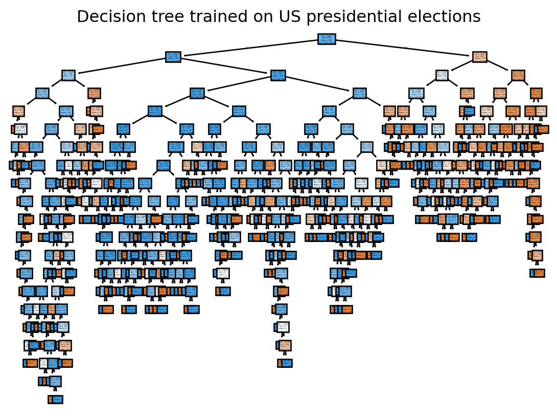
Visualise it with the plot_tree function. What is the problem?
Evaluate its predictive performance. Compare it to that of a tree with a depth of 4. Conclude.
Represent the depth 4 tree with the export_graphviz function.
Look at the following performance metrics: accuracy, f1, recall and precision. Represent the confusion matrix. What is the problem? What solution do you see?
[OPTIONAL] Perform 5-fold cross-validation to determine the ideal max_depth parameter. Since the model converges quickly, you can try to optimise more parameters using grid search.

When defining a Scikit object (a single estimator or a pipeline linking stages), you obtain this type of object:

DecisionTreeClassifier()

In a Jupyter environment, please rerun this cell to show the HTML representation or trust the notebook.
On GitHub, the HTML representation is unable to render, please try loading this page with nbviewer.org.

Figure 2.1 shows that our decision tree obtained initialy needs some pruning. We will test, arbitrarily, a depth-4 tree.

Figure 2.1: Non pruned decision tree (question 4)

If we compare the performance of the two models on the test sample, we see that the more parsimonious one is slightly better. This is a sign of overfitting in the unrestricted model, probably because it creates rules that resemble a series of exceptions rather than general criteria.

	model	performance
0	No restriction	0.843548
1	max_depth = 4	0.854839

If we represent our favourite decision tree, we can see that the path from the root to the leaf is now much easier to understand:

Figure 2.2: Decision tree with max_depth=4 parameter (question 6)

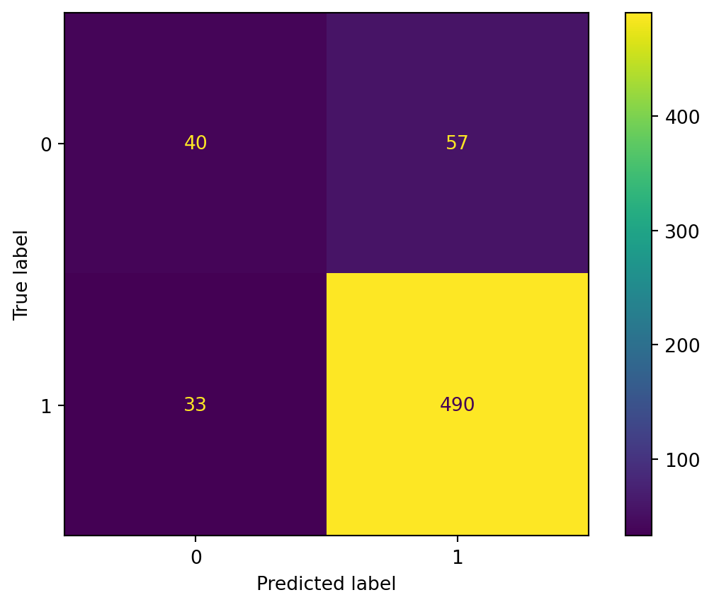
Now, if we represent the confusion matrix, we see that our model is not too bad overall but tends to overpredict class 1 (Republican victory). Why does it do this? Because on average it is a winning bet since we have a class imbalance. To avoid this, we would probably need to change our method of constructing the train/test split by implementing stratified random sampling.

Figure 2.3: Confusion matrix from max_depth=4 decision tree (question 7)

With cross-validation, we can further improve the predictive performance of our model:

GridSearchCV(cv=StratifiedKFold(n_splits=5, random_state=42, shuffle=True),
             estimator=DecisionTreeClassifier(random_state=42), n_jobs=-1,
             param_grid={'criterion': ['gini', 'entropy'],
                         'max_depth': [2, 3, 4, 5, 8, 10],
                         'min_samples_leaf': [1, 2, 5, 10],
                         'min_samples_split': [2, 5, 10]},
             scoring='f1')

In a Jupyter environment, please rerun this cell to show the HTML representation or trust the notebook.
On GitHub, the HTML representation is unable to render, please try loading this page with nbviewer.org.

	param_max_depth	param_min_samples_leaf	param_min_samples_split	param_criterion	mean_test_score	std_test_score	rank_test_score
118	5	10	5	entropy	0.926100	0.002731	1
119	5	10	10	entropy	0.926100	0.002731	1
117	5	10	2	entropy	0.926100	0.002731	1
34	4	10	5	gini	0.925483	0.003617	4
33	4	10	2	gini	0.925483	0.003617	4
35	4	10	10	gini	0.925483	0.003617	4
26	4	1	10	gini	0.924941	0.003441	7
28	4	2	5	gini	0.924941	0.003441	7
27	4	2	2	gini	0.924941	0.003441	7
29	4	2	10	gini	0.924941	0.003441	7

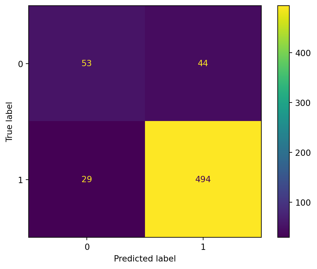
This shows us that we were not so far off from the optimal parameter when we arbitrarily chose max_depth=4. It is already a little better when we look at the confusion matrix, but we are still working with a model that overpredicts the dominant class.

Figure 2.4: Confusion matrix for the best fitting model

If we look at the decision tree (?@fig-decision-treeCV) that this ultimately gives us, we can conclude that:

The variables of educational attainment and income allow us to better distinguish between classes
The unemployment rate variable is only secondary

To go further, we would need to incorporate more variables into the model. But how can we do this without risking overfitting? This will be the subject of the chapter on variable selection.

Figure 2.5: Decision tree the best fitting model

3 Conclusion

We have just briefly looked at the general approach when adopting machine learning. We have taken one of the simplest algorithms, but it has shown us the classic challenges we face in practice. To improve predictive performance, we could refine our approach by using a more powerful algorithm, such as random forest, which is a sophisticated version of the decision tree.

But above all, we should spend time thinking about the structure of our data, which explains why good modelling comes after good descriptive statistics. Without the latter, we are flying blind.

Informations additionnelles

Python environment

This site was built automatically through a Github action using the Quarto reproducible publishing software (version 1.8.26).

The environment used to obtain the results is reproducible via uv. The pyproject.toml file used to build this environment is available on the linogaliana/python-datascientist repository

pyproject.toml

[project]
name = "python-datascientist"
version = "0.1.0"
description = "Source code for Lino Galiana's Python for data science course"
readme = "README.md"
requires-python = ">=3.13,<3.14"
dependencies = [
    "altair>=6.0.0",
    "black==24.8.0",
    "cartiflette",
    "contextily==1.6.2",
    "duckdb>=0.10.1",
    "folium>=0.19.6",
    "gdal!=3.11.1",
    "geoplot==0.5.1",
    "graphviz==0.20.3",
    "great-tables>=0.12.0",
    "gt-extras>=0.0.8",
    "ipykernel>=6.29.5",
    "jupyter>=1.1.1",
    "jupyter-cache==1.0.0",
    "kaleido==0.2.1",
    "langchain-community>=0.3.27",
    "loguru==0.7.3",
    "markdown>=3.8",
    "nbclient==0.10.0",
    "nbformat==5.10.4",
    "nltk>=3.9.1",
    "pip>=25.1.1",
    "plotly>=6.1.2",
    "plotnine>=0.15",
    "polars==1.8.2",
    "pyarrow>=17.0.0",
    "pynsee==0.1.8",
    "python-dotenv==1.0.1",
    "python-frontmatter>=1.1.0",
    "pywaffle==1.1.1",
    "requests>=2.32.3",
    "scikit-image==0.24.0",
    "scipy>=1.13.0",
    "selenium<4.39.0",
    "spacy>=3.8.4",
    "webdriver-manager==4.0.2",
    "wordcloud==1.9.3",
]

[tool.uv.sources]
cartiflette = { git = "https://github.com/inseefrlab/cartiflette" }
gdal = [
  { index = "gdal-wheels", marker = "sys_platform == 'linux'" },
  { index = "geospatial_wheels", marker = "sys_platform == 'win32'" },
]

[[tool.uv.index]]
name = "geospatial_wheels"
url = "https://nathanjmcdougall.github.io/geospatial-wheels-index/"
explicit = true

[[tool.uv.index]]
name = "gdal-wheels"
url = "https://gitlab.com/api/v4/projects/61637378/packages/pypi/simple"
explicit = true

[dependency-groups]
dev = [
    "nb-clean>=4.0.1",
]

To use exactly the same environment (version of Python and packages), please refer to the documentation for uv.

File history

md`This file has been modified __${table_commit.length}__ times since its creation on ${creation_string} (last modified on ${last_modification_string})`

html`<div>${git_history_table}</div>`

html`<div>${git_history_plot}</div>`

SHA	Date	Author	Description
dfae2749	2025-12-25 15:18:33	lgaliana	Details in new classification chapter
8c2b986d	2025-12-25 11:31:10	lgaliana	Forgot to change chapter name
9a1f85b6	2025-12-25 12:29:25	Lino Galiana	Decision tree rather than SVM (#668)
3e04ed3c	2025-11-24 20:08:05	lgaliana	Avoid deprecated ravel method and fix notebooks launch url
94648290	2025-07-22 18:57:48	Lino Galiana	Fix boxes now that it is better supported by jupyter (#628)
91431fa2	2025-06-09 17:08:00	Lino Galiana	Improve homepage hero banner (#612)
48dccf14	2025-01-14 21:45:34	lgaliana	Fix bug in modeling section
8c8ca4c0	2024-12-20 10:45:00	lgaliana	Traduction du chapitre clustering
a5ecaedc	2024-12-20 09:36:42	Lino Galiana	Traduction du chapitre modélisation (#582)
ff0820bc	2024-11-27 15:10:39	lgaliana	Mise en forme chapitre régression
bb943aab	2024-11-26 15:18:41	Lino Galiana	hope works (#579)
e7fd1ff3	2024-11-25 18:20:32	lgaliana	rename classification chapter

creation = d3.min(
  table_commit.map(d => new Date(d.Date))
)

last_modification = d3.max(
  table_commit.map(d => new Date(d.Date))
)

creation_string = creation.toLocaleString("fr", {
  "day": "numeric",
  "month": "long",
  "year": "numeric"
})

last_modification_string = last_modification.toLocaleString("fr", {
  "day": "numeric",
  "month": "long",
  "year": "numeric"
})

git_history_table = Inputs.table(
  table_commit,
  {
    format: {
      SHA: x => md`[${x}](${github_repo}/commit/${x})`,
      Description: x => md`${replacePullRequestPattern(x, github_repo)}`,
      /*Date: x => x.toLocaleString("fr", {
        "month": "numeric",
        "day": "numeric",
        "year": "numeric"
        })
      */
    }
  }
)

git_history_plot = Plot.plot({
  marks: [
    Plot.ruleY([0], {stroke: "royalblue"}),
    Plot.dot(
          table_commit,
          Plot.pointerX({x: (d) => new Date(d.date), y: 0, stroke: "red"})),
    Plot.dot(table_commit, {x: (d) => new Date(d.Date), y: 0, fill: "royalblue"})
  ]
})

function replacePullRequestPattern(inputString, githubRepo) {
    // Use a regular expression to match the pattern #digit
    var pattern = /#(\d+)/g;

    // Replace the pattern with ${github_repo}/pull/#digit
    var replacedString = inputString.replace(pattern, '[#$1](' + githubRepo + '/pull/$1)');

    return replacedString;
}

github_repo = "https://github.com/linogaliana/python-datascientist"

table_commit = {

// Get the HTML table by its class name
var table = document.querySelector('.commit-table');

// Check if the table exists
if (table) {
    // Initialize an array to store the table data
    var dataArray = [];

    // Extract headers from the first row
    var headers = [];
    for (var i = 0; i < table.rows[0].cells.length; i++) {
        headers.push(table.rows[0].cells[i].textContent.trim());
    }

    // Iterate through the rows, starting from the second row
    for (var i = 1; i < table.rows.length; i++) {
        var row = table.rows[i];
        var rowData = {};

        // Iterate through the cells in the row
        for (var j = 0; j < row.cells.length; j++) {
            // Use headers as keys and cell content as values
            rowData[headers[j]] = row.cells[j].textContent.trim();
        }

        // Push the rowData object to the dataArray
        dataArray.push(rowData);
    }
  }

  return dataArray

}

// Get the element with class 'git-details'
{
  var gitDetails = document.querySelector('.commit-table');

  // Check if the element exists
  if (gitDetails) {
      // Hide the element
      gitDetails.style.display = 'none';
  }
}

Plot = require('@observablehq/plot@0.6.12/dist/plot.umd.min.js')

Back to top

Citation

BibTeX citation:

@book{galiana2025,
  author = {Galiana, Lino},
  title = {Python Pour La Data Science},
  date = {2025},
  url = {https://pythonds.linogaliana.fr/},
  doi = {10.5281/zenodo.8229676},
  langid = {en}
}

For attribution, please cite this work as:

Galiana, Lino. 2025. Python Pour La Data Science. https://doi.org/10.5281/zenodo.8229676.

	criterion criterion: {"gini", "entropy", "log_loss"}, default="gini" The function to measure the quality of a split. Supported criteria are "gini" for the Gini impurity and "log_loss" and "entropy" both for the Shannon information gain, see :ref:`tree_mathematical_formulation`.	'gini'
	splitter splitter: {"best", "random"}, default="best" The strategy used to choose the split at each node. Supported strategies are "best" to choose the best split and "random" to choose the best random split.	'best'
	max_depth max_depth: int, default=None The maximum depth of the tree. If None, then nodes are expanded until all leaves are pure or until all leaves contain less than min_samples_split samples.	None
	min_samples_split min_samples_split: int or float, default=2 The minimum number of samples required to split an internal node: - If int, then consider `min_samples_split` as the minimum number. - If float, then `min_samples_split` is a fraction and `ceil(min_samples_split * n_samples)` are the minimum number of samples for each split. .. versionchanged:: 0.18 Added float values for fractions.	2
	min_samples_leaf min_samples_leaf: int or float, default=1 The minimum number of samples required to be at a leaf node. A split point at any depth will only be considered if it leaves at least ``min_samples_leaf`` training samples in each of the left and right branches. This may have the effect of smoothing the model, especially in regression. - If int, then consider `min_samples_leaf` as the minimum number. - If float, then `min_samples_leaf` is a fraction and `ceil(min_samples_leaf * n_samples)` are the minimum number of samples for each node. .. versionchanged:: 0.18 Added float values for fractions.	1
	min_weight_fraction_leaf min_weight_fraction_leaf: float, default=0.0 The minimum weighted fraction of the sum total of weights (of all the input samples) required to be at a leaf node. Samples have equal weight when sample_weight is not provided.	0.0
	max_features max_features: int, float or {"sqrt", "log2"}, default=None The number of features to consider when looking for the best split: - If int, then consider `max_features` features at each split. - If float, then `max_features` is a fraction and `max(1, int(max_features * n_features_in_))` features are considered at each split. - If "sqrt", then `max_features=sqrt(n_features)`. - If "log2", then `max_features=log2(n_features)`. - If None, then `max_features=n_features`. .. note:: The search for a split does not stop until at least one valid partition of the node samples is found, even if it requires to effectively inspect more than ``max_features`` features.	None
	random_state random_state: int, RandomState instance or None, default=None Controls the randomness of the estimator. The features are always randomly permuted at each split, even if ``splitter`` is set to ``"best"``. When ``max_features < n_features``, the algorithm will select ``max_features`` at random at each split before finding the best split among them. But the best found split may vary across different runs, even if ``max_features=n_features``. That is the case, if the improvement of the criterion is identical for several splits and one split has to be selected at random. To obtain a deterministic behaviour during fitting, ``random_state`` has to be fixed to an integer. See :term:`Glossary ` for details.	None
	max_leaf_nodes max_leaf_nodes: int, default=None Grow a tree with ``max_leaf_nodes`` in best-first fashion. Best nodes are defined as relative reduction in impurity. If None then unlimited number of leaf nodes.	None
	min_impurity_decrease min_impurity_decrease: float, default=0.0 A node will be split if this split induces a decrease of the impurity greater than or equal to this value. The weighted impurity decrease equation is the following:: N_t / N * (impurity - N_t_R / N_t * right_impurity - N_t_L / N_t * left_impurity) where ``N`` is the total number of samples, ``N_t`` is the number of samples at the current node, ``N_t_L`` is the number of samples in the left child, and ``N_t_R`` is the number of samples in the right child. ``N``, ``N_t``, ``N_t_R`` and ``N_t_L`` all refer to the weighted sum, if ``sample_weight`` is passed. .. versionadded:: 0.19	0.0
	class_weight class_weight: dict, list of dict or "balanced", default=None Weights associated with classes in the form ``{class_label: weight}``. If None, all classes are supposed to have weight one. For multi-output problems, a list of dicts can be provided in the same order as the columns of y. Note that for multioutput (including multilabel) weights should be defined for each class of every column in its own dict. For example, for four-class multilabel classification weights should be [{0: 1, 1: 1}, {0: 1, 1: 5}, {0: 1, 1: 1}, {0: 1, 1: 1}] instead of [{1:1}, {2:5}, {3:1}, {4:1}]. The "balanced" mode uses the values of y to automatically adjust weights inversely proportional to class frequencies in the input data as ``n_samples / (n_classes * np.bincount(y))`` For multi-output, the weights of each column of y will be multiplied. Note that these weights will be multiplied with sample_weight (passed through the fit method) if sample_weight is specified.	None
	ccp_alpha ccp_alpha: non-negative float, default=0.0 Complexity parameter used for Minimal Cost-Complexity Pruning. The subtree with the largest cost complexity that is smaller than ``ccp_alpha`` will be chosen. By default, no pruning is performed. See :ref:`minimal_cost_complexity_pruning` for details. See :ref:`sphx_glr_auto_examples_tree_plot_cost_complexity_pruning.py` for an example of such pruning. .. versionadded:: 0.22	0.0
	monotonic_cst monotonic_cst: array-like of int of shape (n_features), default=None Indicates the monotonicity constraint to enforce on each feature. - 1: monotonic increase - 0: no constraint - -1: monotonic decrease If monotonic_cst is None, no constraints are applied. Monotonicity constraints are not supported for: - multiclass classifications (i.e. when `n_classes > 2`), - multioutput classifications (i.e. when `n_outputs_ > 1`), - classifications trained on data with missing values. The constraints hold over the probability of the positive class. Read more in the :ref:`User Guide `. .. versionadded:: 1.4	None

	estimator estimator: estimator object This is assumed to implement the scikit-learn estimator interface. Either estimator needs to provide a ``score`` function, or ``scoring`` must be passed.	DecisionTreeC...ndom_state=42)
	param_grid param_grid: dict or list of dictionaries Dictionary with parameters names (`str`) as keys and lists of parameter settings to try as values, or a list of such dictionaries, in which case the grids spanned by each dictionary in the list are explored. This enables searching over any sequence of parameter settings.	{'criterion': ['gini', 'entropy'], 'max_depth': [2, 3, ...], 'min_samples_leaf': [1, 2, ...], 'min_samples_split': [2, 5, ...]}
	scoring scoring: str, callable, list, tuple or dict, default=None Strategy to evaluate the performance of the cross-validated model on the test set. If `scoring` represents a single score, one can use: - a single string (see :ref:`scoring_string_names`); - a callable (see :ref:`scoring_callable`) that returns a single value; - `None`, the `estimator`'s :ref:`default evaluation criterion ` is used. If `scoring` represents multiple scores, one can use: - a list or tuple of unique strings; - a callable returning a dictionary where the keys are the metric names and the values are the metric scores; - a dictionary with metric names as keys and callables as values. See :ref:`multimetric_grid_search` for an example.	'f1'
	n_jobs n_jobs: int, default=None Number of jobs to run in parallel. ``None`` means 1 unless in a :obj:`joblib.parallel_backend` context. ``-1`` means using all processors. See :term:`Glossary ` for more details. .. versionchanged:: v0.20 `n_jobs` default changed from 1 to None	-1
	refit refit: bool, str, or callable, default=True Refit an estimator using the best found parameters on the whole dataset. For multiple metric evaluation, this needs to be a `str` denoting the scorer that would be used to find the best parameters for refitting the estimator at the end. Where there are considerations other than maximum score in choosing a best estimator, ``refit`` can be set to a function which returns the selected ``best_index_`` given ``cv_results_``. In that case, the ``best_estimator_`` and ``best_params_`` will be set according to the returned ``best_index_`` while the ``best_score_`` attribute will not be available. The refitted estimator is made available at the ``best_estimator_`` attribute and permits using ``predict`` directly on this ``GridSearchCV`` instance. Also for multiple metric evaluation, the attributes ``best_index_``, ``best_score_`` and ``best_params_`` will only be available if ``refit`` is set and all of them will be determined w.r.t this specific scorer. See ``scoring`` parameter to know more about multiple metric evaluation. See :ref:`sphx_glr_auto_examples_model_selection_plot_grid_search_digits.py` to see how to design a custom selection strategy using a callable via `refit`. See :ref:`this example ` for an example of how to use ``refit=callable`` to balance model complexity and cross-validated score. .. versionchanged:: 0.20 Support for callable added.	True
	cv cv: int, cross-validation generator or an iterable, default=None Determines the cross-validation splitting strategy. Possible inputs for cv are: - None, to use the default 5-fold cross validation, - integer, to specify the number of folds in a `(Stratified)KFold`, - :term:`CV splitter`, - An iterable yielding (train, test) splits as arrays of indices. For integer/None inputs, if the estimator is a classifier and ``y`` is either binary or multiclass, :class:`StratifiedKFold` is used. In all other cases, :class:`KFold` is used. These splitters are instantiated with `shuffle=False` so the splits will be the same across calls. Refer :ref:`User Guide ` for the various cross-validation strategies that can be used here. .. versionchanged:: 0.22 ``cv`` default value if None changed from 3-fold to 5-fold.	StratifiedKFo... shuffle=True)
	verbose verbose: int Controls the verbosity: the higher, the more messages. - >1 : the computation time for each fold and parameter candidate is displayed; - >2 : the score is also displayed; - >3 : the fold and candidate parameter indexes are also displayed together with the starting time of the computation.	0
	pre_dispatch pre_dispatch: int, or str, default='2n_jobs' Controls the number of jobs that get dispatched during parallel execution. Reducing this number can be useful to avoid an explosion of memory consumption when more jobs get dispatched than CPUs can process. This parameter can be: - None, in which case all the jobs are immediately created and spawned. Use this for lightweight and fast-running jobs, to avoid delays due to on-demand spawning of the jobs - An int, giving the exact number of total jobs that are spawned - A str, giving an expression as a function of n_jobs, as in '2n_jobs'	'2*n_jobs'
	error_score error_score: 'raise' or numeric, default=np.nan Value to assign to the score if an error occurs in estimator fitting. If set to 'raise', the error is raised. If a numeric value is given, FitFailedWarning is raised. This parameter does not affect the refit step, which will always raise the error.	nan
	return_train_score return_train_score: bool, default=False If ``False``, the ``cv_results_`` attribute will not include training scores. Computing training scores is used to get insights on how different parameter settings impact the overfitting/underfitting trade-off. However computing the scores on the training set can be computationally expensive and is not strictly required to select the parameters that yield the best generalization performance. .. versionadded:: 0.19 .. versionchanged:: 0.21 Default value was changed from ``True`` to ``False``	False

	criterion criterion: {"gini", "entropy", "log_loss"}, default="gini" The function to measure the quality of a split. Supported criteria are "gini" for the Gini impurity and "log_loss" and "entropy" both for the Shannon information gain, see :ref:`tree_mathematical_formulation`.	'entropy'
	splitter splitter: {"best", "random"}, default="best" The strategy used to choose the split at each node. Supported strategies are "best" to choose the best split and "random" to choose the best random split.	'best'
	max_depth max_depth: int, default=None The maximum depth of the tree. If None, then nodes are expanded until all leaves are pure or until all leaves contain less than min_samples_split samples.	5
	min_samples_split min_samples_split: int or float, default=2 The minimum number of samples required to split an internal node: - If int, then consider `min_samples_split` as the minimum number. - If float, then `min_samples_split` is a fraction and `ceil(min_samples_split * n_samples)` are the minimum number of samples for each split. .. versionchanged:: 0.18 Added float values for fractions.	2
	min_samples_leaf min_samples_leaf: int or float, default=1 The minimum number of samples required to be at a leaf node. A split point at any depth will only be considered if it leaves at least ``min_samples_leaf`` training samples in each of the left and right branches. This may have the effect of smoothing the model, especially in regression. - If int, then consider `min_samples_leaf` as the minimum number. - If float, then `min_samples_leaf` is a fraction and `ceil(min_samples_leaf * n_samples)` are the minimum number of samples for each node. .. versionchanged:: 0.18 Added float values for fractions.	10
	min_weight_fraction_leaf min_weight_fraction_leaf: float, default=0.0 The minimum weighted fraction of the sum total of weights (of all the input samples) required to be at a leaf node. Samples have equal weight when sample_weight is not provided.	0.0
	max_features max_features: int, float or {"sqrt", "log2"}, default=None The number of features to consider when looking for the best split: - If int, then consider `max_features` features at each split. - If float, then `max_features` is a fraction and `max(1, int(max_features * n_features_in_))` features are considered at each split. - If "sqrt", then `max_features=sqrt(n_features)`. - If "log2", then `max_features=log2(n_features)`. - If None, then `max_features=n_features`. .. note:: The search for a split does not stop until at least one valid partition of the node samples is found, even if it requires to effectively inspect more than ``max_features`` features.	None
	random_state random_state: int, RandomState instance or None, default=None Controls the randomness of the estimator. The features are always randomly permuted at each split, even if ``splitter`` is set to ``"best"``. When ``max_features < n_features``, the algorithm will select ``max_features`` at random at each split before finding the best split among them. But the best found split may vary across different runs, even if ``max_features=n_features``. That is the case, if the improvement of the criterion is identical for several splits and one split has to be selected at random. To obtain a deterministic behaviour during fitting, ``random_state`` has to be fixed to an integer. See :term:`Glossary ` for details.	42
	max_leaf_nodes max_leaf_nodes: int, default=None Grow a tree with ``max_leaf_nodes`` in best-first fashion. Best nodes are defined as relative reduction in impurity. If None then unlimited number of leaf nodes.	None
	min_impurity_decrease min_impurity_decrease: float, default=0.0 A node will be split if this split induces a decrease of the impurity greater than or equal to this value. The weighted impurity decrease equation is the following:: N_t / N * (impurity - N_t_R / N_t * right_impurity - N_t_L / N_t * left_impurity) where ``N`` is the total number of samples, ``N_t`` is the number of samples at the current node, ``N_t_L`` is the number of samples in the left child, and ``N_t_R`` is the number of samples in the right child. ``N``, ``N_t``, ``N_t_R`` and ``N_t_L`` all refer to the weighted sum, if ``sample_weight`` is passed. .. versionadded:: 0.19	0.0
	class_weight class_weight: dict, list of dict or "balanced", default=None Weights associated with classes in the form ``{class_label: weight}``. If None, all classes are supposed to have weight one. For multi-output problems, a list of dicts can be provided in the same order as the columns of y. Note that for multioutput (including multilabel) weights should be defined for each class of every column in its own dict. For example, for four-class multilabel classification weights should be [{0: 1, 1: 1}, {0: 1, 1: 5}, {0: 1, 1: 1}, {0: 1, 1: 1}] instead of [{1:1}, {2:5}, {3:1}, {4:1}]. The "balanced" mode uses the values of y to automatically adjust weights inversely proportional to class frequencies in the input data as ``n_samples / (n_classes * np.bincount(y))`` For multi-output, the weights of each column of y will be multiplied. Note that these weights will be multiplied with sample_weight (passed through the fit method) if sample_weight is specified.	None
	ccp_alpha ccp_alpha: non-negative float, default=0.0 Complexity parameter used for Minimal Cost-Complexity Pruning. The subtree with the largest cost complexity that is smaller than ``ccp_alpha`` will be chosen. By default, no pruning is performed. See :ref:`minimal_cost_complexity_pruning` for details. See :ref:`sphx_glr_auto_examples_tree_plot_cost_complexity_pruning.py` for an example of such pruning. .. versionadded:: 0.22	0.0
	monotonic_cst monotonic_cst: array-like of int of shape (n_features), default=None Indicates the monotonicity constraint to enforce on each feature. - 1: monotonic increase - 0: no constraint - -1: monotonic decrease If monotonic_cst is None, no constraints are applied. Monotonicity constraints are not supported for: - multiclass classifications (i.e. when `n_classes > 2`), - multioutput classifications (i.e. when `n_outputs_ > 1`), - classifications trained on data with missing values. The constraints hold over the probability of the positive class. Read more in the :ref:`User Guide `. .. versionadded:: 1.4	None