Python pour la data science

Lino Galiana

doi:10.5281/zenodo.8229676

If you want to try the examples in this tutorial:

Skills to be acquired by the end of this chapter

How to construct fine aggregate statistics using Pandas methods;
Know how to reshape your data from long to wide format (and vice versa);
Create attractive tables to communicate aggregated results.

1 Introduction

The previous chapter showed how to enrich a dataset by associating it with another source through a join. We now have two datasets that have been made consistent with one another: the Ademe greenhouse gas emissions data (emissions) and the Insee Filosofi framing data (filosofi).

This chapter will use this association to deepen our understanding of the data through two complementary operations:

group descriptive statistics;
reshaping data between long and wide formats.

Finally, we will see how to build, from these statistics, polished communication tables using the great_tables package.

1.1 Data

We start again from the same datasets as in the chapter on joins: the Ademe municipal emissions data (emissions) and the Insee Filosofi data (filosofi), enriched with one another. The code below, already explained in detail in the previous chapter, retrieves these datasets again:

See data retrieval code

import requests
import pandas as pd

def get_melodi(dataset, dimension, code, value_name, time_period, geo_level="COM"):

  url = f"https://api.insee.fr/melodi/data/{dataset}"

  params = {
    "GEO": geo_level,
    dimension: code,
    "TIME_PERIOD": time_period,
    "maxResult": 40000,
  }

  response = requests.get(url, params=params, timeout=60)
  response.raise_for_status()
  observations = response.json()["observations"]

  return pd.DataFrame(
    {
      "CODGEO": obs["dimensions"]["GEO"].split("-")[-1],
      value_name: obs["measures"]["OBS_VALUE_NIVEAU"].get("value"),
    }
    for obs in observations
  )

niveau_vie = get_melodi("DS_FILOSOFI_CC", "FILOSOFI_MEASURE", "MED_SL", "NIVVIE_MEDIAN", 2023)
taux_pauvrete = get_melodi("DS_FILOSOFI_CC", "FILOSOFI_MEASURE", "PR_MD60", "TAUX_PAUVRETE", 2023)
population = get_melodi("DS_POPULATIONS_HISTORIQUES", "POPREF_MEASURE", "PMUN", "POPULATION", 2023)

url_cog_2023 = "https://www.insee.fr/fr/statistiques/fichier/6800675/v_commune_2023.csv"
url_backup = "https://minio.lab.sspcloud.fr/lgaliana/data/python-ENSAE/cog_2023.csv"

try:
  cog_2023 = pd.read_csv(url_cog_2023)
except requests.exceptions.Timeout:
  cog_2023 = pd.read_csv(url_backup)

noms_communes = (
  cog_2023
  .loc[cog_2023["TYPECOM"] == "COM", ["COM", "LIBELLE"]]
  .rename(columns={"COM": "CODGEO", "LIBELLE": "LIBGEO"})
)

filosofi = (
  niveau_vie
  .merge(taux_pauvrete, on="CODGEO", how="outer")
  .merge(population, on="CODGEO", how="outer")
  .merge(noms_communes, on="CODGEO", how="left")
  [["CODGEO", "LIBGEO", "POPULATION", "NIVVIE_MEDIAN", "TAUX_PAUVRETE"]]
)

filosofi["POPULATION"] = filosofi["POPULATION"].astype(int)
filosofi["dep"] = filosofi["CODGEO"].str[:2]

import pandas as pd

url = "https://data.ademe.fr/data-fair/api/v1/datasets/igt-pouvoir-de-rechauffement-global/convert"
emissions = pd.read_csv(url)
emissions["dep"] = emissions["INSEE commune"].str[:2]

emissions.head(2)

	INSEE commune	Commune	Agriculture	Autres transports	Autres transports international	CO2 biomasse hors-total	Déchets	Energie	Industrie hors-énergie	Résidentiel	Routier	Tertiaire	dep
0	01001	L'ABERGEMENT-CLEMENCIAT	3711.425991	NaN	NaN	432.751835	101.430476	2.354558	6.911213	309.358195	793.156501	367.036172	01
1	01002	L'ABERGEMENT-DE-VAREY	475.330205	NaN	NaN	140.741660	140.675439	2.354558	6.911213	104.866444	348.997893	112.934207	01

We will also need the following packages

To obtain reproducible results, you can set the seed of the pseudo-random number generator.

np.random.seed(123)

2 Descriptive statistics by group

2.1 Principle

In the introductory chapter, we saw how to obtain an aggregated statistic easily with Pandas. However, it is common to have data with intermediate analysis strata that are relevant: geographical variables, membership in socio-demographic groups related to recorded characteristics, temporal period indicators, etc. To better understand the structure of the data, data scientists are often led to construct descriptive statistics on sub-groups present in the data.

For example, we previously constructed emission statistics at the national level. But what about the emission profiles of different departments? To answer this question, it will be useful to aggregate our data at the departmental level. This will give us different information from the initial dataset (municipal level) and the most aggregated level (national level).

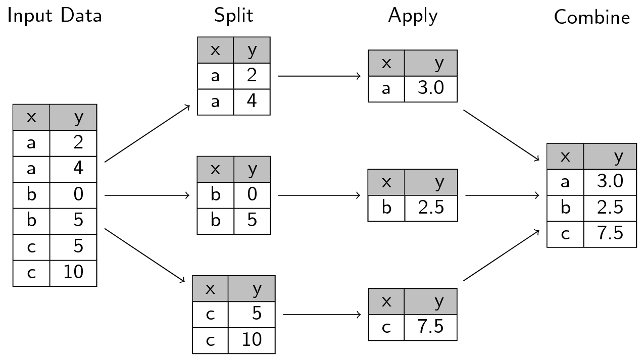
In SQL, it is very simple to segment data to perform operations on coherent blocks and recollect results in the appropriate dimension. The underlying logic is that of split-apply-combine, which is adopted by data manipulation languages, including pandas which is no exception.

The following image, from this site, well represents how the split-apply-combine approach works:

Split-apply-combine (Source: unlhcc.github.io)

In Pandas, we use groupby to segment the data according to one or more axes (this tutorial on the subject is particularly useful). All the aggregation operations (counting, averages, etc.) that we saw earlier can be applied by group.

Technically, this operation involves creating an association between labels (values of group variables) and observations. Using the groupby method does not trigger operations until a statistic is implemented; it simply creates a formal relationship between observations and groupings that will be used later:

filosofi.groupby('dep').__class__

pandas.api.typing.DataFrameGroupBy

As long as we do not call an action on a DataFrame by group, such as head or display, pandas performs no operations. This is called lazy evaluation. For example, the result of df.groupby('dep') is a transformation that has not yet been evaluated:

filosofi.groupby('dep')

<pandas.api.typing.DataFrameGroupBy object at 0x7fce50e7d590>

2.2 Illustration 1: counting by group

To illustrate the application of this principle to counting, we can count the number of municipalities by department in 2023 (this statistic changes every year due to municipal mergers). For this, we simply take the reference of French municipalities from the official geographical code (COG) and count by department using count:

With this dataset, without resorting to group statistics, we can already know how many municipalities, departments, and regions we have in France, respectively:

1communes = cog_2023.loc[cog_2023['TYPECOM']=="COM"]
communes.loc[:, ['COM', 'DEP', 'REG']].nunique()

1: We restrict to the status “Commune” because this file also contains Insee codes for other statuses, such as the “Municipal Arrondissements” of Paris, Lyon, and Marseille.

COM    34945
DEP      101
REG       18
dtype: int64

Now, let’s look at the departments with the most municipalities. It is the same counting function where we play, this time, on the group from which the statistic is calculated.

Calculating this statistic is quite straightforward when you understand the principle of calculating statistics with Pandas:

communes = cog_2023.loc[cog_2023['TYPECOM']=="COM"]
communes.groupby('DEP').agg({'COM': 'nunique'})

	COM
DEP
01	392
02	798
03	317
04	198
05	162
...	...
971	32
972	34
973	22
974	24
976	17

101 rows × 1 columns

In SQL, we would use the following query:

SELECT dep, COUNT DISTINCT "COM" AS COM
FROM communes
GROUP BY dep
WHERE TYPECOM == 'COM';

The output is an indexed Series. This is not very convenient as we mentioned in the previous chapter. It is more practical to transform this object into a DataFrame with reset_index. Finally, with sort_values, we obtain the desired statistic:

(
    communes
    .groupby('DEP')
    .agg({'COM': 'nunique'})
    .reset_index()
    .sort_values('COM', ascending = False)
)

	DEP	COM
62	62	890
1	02	798
80	80	772
57	57	725
76	76	708
...	...	...
96	971	32
99	974	24
98	973	22
100	976	17
75	75	1

101 rows × 2 columns

2.3 Illustration 2: aggregates by group

To illustrate aggregates by group, we can use the Insee filosofi dataset and sum the POPULATION variable.

To calculate the total for the whole of France, we can do it in two ways:

filosofi['POPULATION'].sum()* 1e-6

np.float64(68.09428)

filosofi.agg({"POPULATION": "sum"}).div(1e6)

POPULATION    68.09428
dtype: float64

where the results are reported in millions of people. The logic is the same when doing group statistics, it’s just a matter of replacing filosofi with filosofi.groupby('dep') to create a partitioned version of our dataset by department:

1filosofi.groupby('dep')['POPULATION'].sum()

1: With this approach, you need to pay attention to the order of operations: first, perform the groupby and then select the column of interest

dep
01     679344
02     523342
03     333298
04     168054
05     143467
       ...   
92    1654712
93    1704316
94    1426929
95    1281653
97    1928465
Name: POPULATION, Length: 97, dtype: int64

filosofi.groupby('dep').agg({"POPULATION": "sum"})

	POPULATION
dep
01	679344
02	523342
03	333298
04	168054
05	143467
...	...
92	1654712
93	1704316
94	1426929
95	1281653
97	1928465

97 rows × 1 columns

The second approach is more practical because it directly gives a Pandas DataFrame and not an unnamed indexed series. From this, a few basic manipulations can suffice to have a shareable table on departmental demographics. However, this table would be somewhat rudimentary as we currently only have the department numbers. To get the names of the departments, we would need to use a second dataset and merge the common information between them (in this case, the department number): this is exactly the join principle we implemented in the previous chapter.

3 Application

This application exercise uses the Ademe dataset named emissions previously discussed.

Exercise 1: Group Aggregations

Calculate the total emissions of the “Residential” sector by department and compare the value to the most polluting department in this sector. Draw insights from the reality that this statistic reflects.
Calculate the total emissions for each sector in each department. For each department, calculate the proportion of total emissions coming from each sector.

Hint for this question

“Group by” = groupby
“Total emissions” = agg({*** : "sum"})

In question 1, the result should be as follows:

	dep	Résidentiel	Résidentiel (% valeur max)
59	59	3.498347e+06	1.000000
75	75	1.934580e+06	0.552998
69	69	1.774653e+06	0.507283
62	62	1.738090e+06	0.496832
57	57	1.644192e+06	0.469991

This ranking may reflect demographics rather than the process we wish to measure. Without the addition of information on the population of each département to control for this factor, it is difficult to know whether there is a structural difference in behavior between the inhabitants of Nord (département 59) and Moselle (département 57).

At the end of question 2, let’s take the share of emissions from agriculture and the tertiary sector in departmental emissions:

	Agriculture	Autres transports	Autres transports international	CO2 biomasse hors-total	Déchets	Energie	Industrie hors-énergie	Résidentiel	Routier	Tertiaire	...	Part Agriculture	Part Autres transports	Part Autres transports international	Part CO2 biomasse hors-total	Part Déchets	Part Energie	Part Industrie hors-énergie	Part Résidentiel	Part Routier	Part Tertiaire
dep
23	1.430068e+06	5060.057601	0.000000	210196.604389	26550.858041	9752.578164	28626.245699	134197.515156	434767.868975	70733.245013	...	60.855172	0.215326	0.000000	8.944716	1.129846	0.415012	1.218163	5.710647	18.501132	3.009986
48	7.510594e+05	5697.938112	0.000000	70903.948092	26011.591018	6065.340741	17803.285591	61033.998303	253618.488432	43661.121359	...	60.772448	0.461052	0.000000	5.737238	2.104744	0.490781	1.440564	4.938605	20.521701	3.532867
15	1.539204e+06	8261.874450	18.804572	228415.892777	44814.875202	13138.432196	85214.659284	128315.601994	443832.903418	84364.615635	...	59.761414	0.320777	0.000730	8.868517	1.739990	0.510115	3.308560	4.982005	17.232336	3.275556
12	2.122331e+06	13796.608978	3124.844800	331420.983449	52412.681268	35405.484754	112897.690887	268862.654280	795413.985637	170211.845832	...	54.336847	0.353227	0.080004	8.485186	1.341893	0.906467	2.890457	6.883541	20.364540	4.357839
32	1.026604e+06	4599.824552	0.000000	201732.703762	50950.668326	16651.432346	53468.498055	158218.000190	446345.993580	105662.674213	...	49.732924	0.222835	0.000000	9.772766	2.468261	0.806664	2.590235	7.664734	21.622845	5.118737

5 rows × 21 columns

	Agriculture	Autres transports	Autres transports international	CO2 biomasse hors-total	Déchets	Energie	Industrie hors-énergie	Résidentiel	Routier	Tertiaire	...	Part Agriculture	Part Autres transports	Part Autres transports international	Part CO2 biomasse hors-total	Part Déchets	Part Energie	Part Industrie hors-énergie	Part Résidentiel	Part Routier	Part Tertiaire
dep
75	0.000000	42216.829025	1.837660e+02	1.186577e+06	27358.781206	147965.117571	434314.469384	1.934580e+06	1.625583e+06	1.331630e+06	...	0.000000	0.627255	0.002730	17.630092	0.406495	2.198457	6.453018	28.743870	24.152808	19.785275
94	2259.429643	218992.353559	3.146283e+05	6.914050e+05	213619.661516	76341.230740	467189.038927	1.336894e+06	1.169432e+06	7.636502e+05	...	0.043001	4.167781	5.987888	13.158562	4.065530	1.452898	8.891367	25.443275	22.256193	14.533505
92	91.408184	12340.794839	2.101194e+02	1.067889e+06	264497.880711	242842.018012	706597.424067	1.466794e+06	1.198420e+06	8.360132e+05	...	0.001577	0.212930	0.003625	18.425550	4.563695	4.190041	12.191761	25.308332	20.677765	14.424724
93	2018.470982	59617.086124	1.101400e+06	7.259516e+05	252166.943778	102837.663903	433216.360990	1.316452e+06	1.396911e+06	8.630178e+05	...	0.032277	0.953326	17.612287	11.608558	4.032355	1.644458	6.927483	21.051146	22.337751	13.800359
83	151715.557862	21772.374976	2.854770e+04	5.795888e+05	233522.964403	47044.063669	139710.930613	5.938382e+05	1.944266e+06	5.610540e+05	...	3.527399	0.506209	0.663736	13.475487	5.429428	1.093778	3.248291	13.806786	45.204334	13.044551

5 rows × 21 columns

These results are quite logical; rural departments have a larger share of their emissions from agriculture, while urban departments have higher emissions from the tertiary sector, which is related to the higher density of these areas.

With these statistics, we progress in understanding our dataset and, consequently, the nature of CO2 emissions in France. Descriptive statistics by group help us better grasp the spatial heterogeneity of our phenomenon.

However, we would remain limited in our ability to interpret these statistics without additional information: a département could look like a low emitter simply because it is sparsely populated. This is exactly the kind of limitation we resolved thanks to enriching our data with a join against the Filosofi data (see in particular the computation of a carbon footprint per capita in the previous chapter).

4 Restructuring datasets

4.1 Principle

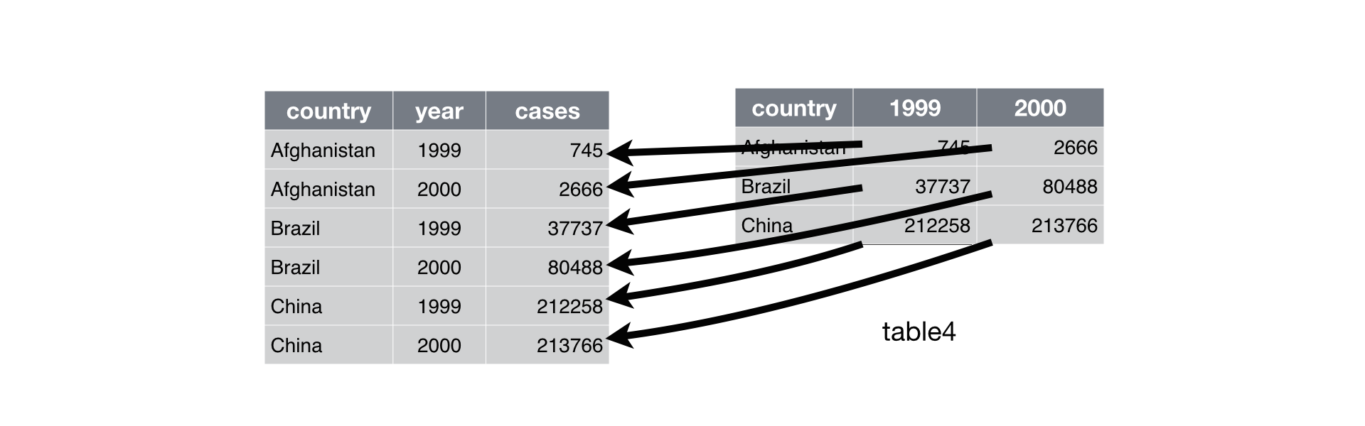
When we have multiple pieces of information for the same individual or group, we generally find two types of data structures:

Wide format: the data contains repeated observations for the same individual (or group) in different columns.
Long format: the data contains repeated observations for the same individual in different rows, with a column distinguishing the observation levels.

An example of the distinction between the two can be taken from Hadley Wickham’s reference book, R for Data Science:

Wide and Long Data Formats (Source: R for Data Science) — Wide and Long Data Formats (Source: *R for Data Science*)

The following cheat sheet will help remember the functions to apply if needed:

Switching from a wide format to a long format (or vice versa) can be extremely practical because certain functions are more suitable for one form of data than the other.

Generally, with Python as with R, long formats are often preferable. Wide formats are rather designed for spreadsheets like Excel, where we have a limited number of rows to create pivot tables from.

4.2 Application

The ADEME data, and the Insee data as well, are in the wide format. The next exercise illustrates the benefit of converting from long to wide before creating a plot with the plot method seen in the introductory chapter.

Exercice 2: Restructuring Data: Wide to Long

Create a copy of the ADEME data by doing df_wide = emissions.copy()
Restructure the data into the long format to have emission data by sector while keeping the commune as the level of analysis (pay attention to other identifying variables).
Sum the emissions by sector and represent it graphically.
For each department, identify the most polluting sector.

5 Formatting descriptive statistics tables

A Pandas DataFrame is automatically formatted when viewed from a notebook as a minimally styled HTML table. This formatting is convenient for viewing data, a necessary task for data scientists, but it doesn’t go much beyond that.

In an exploratory phase, it can be useful to have a more complete table, including minimal visualizations, to better understand the data. In the final phase of a project, when communicating about it, having an attractive visualization is advantageous. The outputs of notebooks are not a satisfactory solution for these needs and require the medium of the notebook, which can deter some users.

Fortunately, the young package great_tables allows for the creation of tables programmatically that rival tedious manual productions in Excel and are difficult to replicate. This package is a Python port of the GT package. great_tables builds HTML tables, offering great formatting richness and excellent integration with Quarto, the reproducible publishing tool developed by RStudio.

The following exercise will propose building a table with this package, step by step. It requires installing the great_tables package beforehand:

!pip install great_tables --quiet

To focus on table construction, the necessary data preparations are provided directly. We will start from the emissions_merged dataset, built in the previous chapter when computing the carbon footprint per capita, which looks like this:

To ensure you are able to complete the next exercise, here is the dataframe required for it.

emissions_totales_commune = emissions.sum(axis = 1, numeric_only = True)

emissions_merged = (
    emissions.assign(emissions = emissions_totales_commune)
    .reset_index()
    .merge(filosofi, left_on = "INSEE commune", right_on = "CODGEO")
)
emissions_merged = emissions_merged.loc[emissions_merged['POPULATION'] > 0]
emissions_merged['empreinte'] = emissions_merged['emissions']/emissions_merged['POPULATION']
emissions_merged['empreinte'] = emissions_merged['empreinte'].astype(float)

emissions_table = (
    emissions_merged
    .rename(columns={"dep_y": "dep", "POPULATION": "population", "NIVVIE_MEDIAN": "revenu"})
    .groupby("dep")
    .agg({"empreinte": "sum", "revenu": "median", "population": "sum"}) #pas vraiment le revenu médian
    .reset_index()
    .sort_values(by = "empreinte")
)

In this table, we will include horizontal bars, similar to the examples shown here. This is done by directly including the HTML code in the DataFrame column.

def create_bar(prop_fill: float, max_width: int, height: int, color: str = "green") -> str:
    """Create divs to represent prop_fill as a bar."""
    width = round(max_width * prop_fill, 2)
    px_width = f"{width}px"
    return f"""\
    <div style="width: {max_width}px; background-color: lightgrey;">\
        <div style="height:{height}px;width:{px_width};background-color:{color};"></div>\
    </div>\
    """

colors = {'empreinte': "green", 'revenu': "red", 'population': "blue"}

for variable in ['empreinte', 'revenu', 'population']:
    emissions_table[f'raw_perc_{variable}'] = emissions_table[variable]/emissions_table[variable].max()
    emissions_table[f'bar_{variable}'] = emissions_table[f'raw_perc_{variable}'].map(
        lambda x: create_bar(x, max_width=75, height=20, color = colors[variable])
    )

We keep only the 5 smallest carbon footprints and the five largest.

emissions_min = emissions_table.head(5).assign(grp = "5 départements les moins pollueurs").reset_index(drop=True)
emissions_max = emissions_table.tail(5).assign(grp = "5 départements les plus pollueurs").reset_index(drop=True)

emissions_table = pd.concat([
    emissions_min,
    emissions_max
])

Finally, to use some practical functions for selecting columns based on patterns, we will convert the data to the Polars format.

import polars as pl
emissions_table = pl.from_pandas(emissions_table)

Exercise 5: A Beautiful Descriptive Statistics Table (Open Exercise)

Using this base table

GT(emissions_table, groupname_col="grp", rowname_col="dep")

construct a table in the style of the one below.

# Start from here
GT(emissions_table, groupname_col="grp", rowname_col="dep")

	empreinte	revenu	population	raw_perc_empreinte	raw_perc_revenu	raw_perc_population
5 départements les moins pollueurs
92	142.01712816633915	36310.0	1654712	0.0077652880870661455	1.0	0.6326234356093262
93	147.9911027308174	21820.0	1704316	0.008091936246460305	0.6009363811622143	0.6515878553391433
94	196.38841932390835	27940.0	1426929	0.010738230470535274	0.7694849903607821	0.5455382727330075
90	895.5043935192521	29170.0	140255	0.04896486563765511	0.8033599559350041	0.05362177826799228
83	922.1520421556788	26130.0	1119307	0.05042191994636078	0.7196364637840815	0.4279293555866931
5 départements les plus pollueurs
52	13068.456519747897	24610.0	168331	0.7145640180125334	0.6777747177086202	0.06435569183009097
55	13651.074978199267	25340.0	180290	0.7464207400370646	0.6978793720738089	0.06892781294026117
51	14401.966686862248	28180.0	563076	0.7874783963581239	0.7760947397411182	0.21527315546702808
21	15405.932865409246	27090.0	540100	0.8423737931792529	0.7460754613054255	0.2064890552389764
77	18288.713383716273	28910.0	1468108	1.0	0.7961993941063068	0.5612816772982469

The table you should have :

	Footprint		Median Income		Population
Carbon Footprint
Initial descriptive statistics to refine
	Carbon Footprint	(%)*	Income	(%)*	Population	(%)*
5 départements les moins pollueurs
92	14.20	0.8%	36.3K	100.0%	1.65M	63.3%
93	14.80	0.8%	21.8K	60.1%	1.70M	65.2%
94	19.64	1.1%	27.9K	76.9%	1.43M	54.6%
90	89.55	4.9%	29.2K	80.3%	140.25K	5.4%
83	92.22	5.0%	26.1K	72.0%	1.12M	42.8%
5 départements les plus pollueurs
52	1,306.85	71.5%	24.6K	67.8%	168.33K	6.4%
55	1,365.11	74.6%	25.3K	69.8%	180.29K	6.9%
51	1,440.20	78.7%	28.2K	77.6%	563.08K	21.5%
21	1,540.59	84.2%	27.1K	74.6%	540.10K	20.6%
77	1,828.87	100.0%	28.9K	79.6%	1.47M	56.1%
*Note: The median income presented here is an approximation of the department's median income.
Reading: The (%) columns presented above are scaled to the maximum value of the variable
Source: Calculations based on Ademe data

Thanks to this, we can already understand that our definition of the carbon footprint is certainly flawed. It seems unlikely that the inhabitants of the 77th department have a carbon footprint 500 times greater than that of intra-muros Paris. The main reason? We are not dealing with a concept of consumption emissions but production emissions, which penalizes industrial areas or areas with airports…

To learn more about constructing tables with great_tables, you can replicate this exercise on producing electoral tables that I proposed for an R course with gt, the equivalent of great_tables for R.

We have now covered the main features of Pandas for manipulating and reshaping data. The last chapter of this part takes a step back to look at the limitations of Pandas syntax and discover the alternative ecosystems that exist to go further.

Informations additionnelles

Python environment

This site was built automatically through a Github action using the Quarto reproducible publishing software (version 1.8.26).

The environment used to obtain the results is reproducible via uv. The pyproject.toml file used to build this environment is available on the linogaliana/python-datascientist repository

pyproject.toml

[project]
name = "python-datascientist"
version = "0.1.0"
description = "Source code for Lino Galiana's Python for data science course"
readme = "README.md"
requires-python = ">=3.13,<3.14"
dependencies = [
    "altair>=6.0.0",
    "cartiflette",
    "contextily==1.6.2",
    "duckdb>=0.10.1",
    "folium>=0.19.6",
    "gdal==3.11.4",
    "graphviz==0.20.3",
    "great-tables>=0.12.0",
    "gt-extras>=0.0.8",
    "ipykernel>=6.29.5",
    "jupyter>=1.1.1",
    "jupyter-cache>=1.0.0",
    "kaleido>=0.2.1",
    "langchain-community>=0.3.27",
    "loguru==0.7.3",
    "markdown>=3.8",
    "nbclient>=0.10.0",
    "nbformat>=5.10.4",
    "nltk>=3.9.1",
    "pandas>=3.0",
    "pip>=25.1.1",
    "plotly>=6.1.2",
    "plotnine>=0.15",
    "polars>=1.8.2",
    "pyarrow>=17.0.0",
    "pynsee>=0.1.8",
    "python-dotenv>=1.0.1",
    "python-frontmatter>=1.1.0",
    "pywaffle>=1.1.1",
    "requests>=2.32.3",
    "scikit-image>=0.24.0",
    "scikit-learn>=1.8.0",
    "scipy>=1.13.0",
    "seaborn>=0.13.2",
    "selenium<4.39.0",
    "spacy>=3.8.4",
    "webdriver-manager>=4.0.2",
    "wordcloud==1.9.3",
]

[tool.uv.sources]
cartiflette = { git = "https://github.com/inseefrlab/cartiflette" }
gdal = [
  { index = "gdal-wheels", marker = "sys_platform == 'linux'" },
  { index = "geospatial_wheels", marker = "sys_platform == 'win32'" },
]

[[tool.uv.index]]
name = "geospatial_wheels"
url = "https://nathanjmcdougall.github.io/geospatial-wheels-index/"
explicit = true

[[tool.uv.index]]
name = "gdal-wheels"
url = "https://gitlab.com/api/v4/projects/61637378/packages/pypi/simple"
explicit = true

[dependency-groups]
dev = [
    "nb-clean>=4.0.1",
]

To use exactly the same environment (version of Python and packages), please refer to the documentation for uv.

File history

md`This file has been modified __${table_commit.length}__ times since its creation on ${creation_string} (last modified on ${last_modification_string})`

html`<div>${git_history_table}</div>`

html`<div>${git_history_plot}</div>`

SHA	Date	Author	Description
56ad5bc8	2026-07-14 21:57:39	Lino Galiana	Données filosofi plus à jour pour le chapitre Pandas (#699)

creation = d3.min(
  table_commit.map(d => new Date(d.Date))
)

last_modification = d3.max(
  table_commit.map(d => new Date(d.Date))
)

creation_string = creation.toLocaleString("fr", {
  "day": "numeric",
  "month": "long",
  "year": "numeric"
})

last_modification_string = last_modification.toLocaleString("fr", {
  "day": "numeric",
  "month": "long",
  "year": "numeric"
})

git_history_table = Inputs.table(
  table_commit,
  {
    format: {
      SHA: x => md`[${x}](${github_repo}/commit/${x})`,
      Description: x => md`${replacePullRequestPattern(x, github_repo)}`,
      /*Date: x => x.toLocaleString("fr", {
        "month": "numeric",
        "day": "numeric",
        "year": "numeric"
        })
      */
    }
  }
)

git_history_plot = Plot.plot({
  marks: [
    Plot.ruleY([0], {stroke: "royalblue"}),
    Plot.dot(
          table_commit,
          Plot.pointerX({x: (d) => new Date(d.date), y: 0, stroke: "red"})),
    Plot.dot(table_commit, {x: (d) => new Date(d.Date), y: 0, fill: "royalblue"})
  ]
})

function replacePullRequestPattern(inputString, githubRepo) {
    // Use a regular expression to match the pattern #digit
    var pattern = /#(\d+)/g;

    // Replace the pattern with ${github_repo}/pull/#digit
    var replacedString = inputString.replace(pattern, '[#$1](' + githubRepo + '/pull/$1)');

    return replacedString;
}

github_repo = "https://github.com/linogaliana/python-datascientist"

table_commit = {

// Get the HTML table by its class name
var table = document.querySelector('.commit-table');

// Check if the table exists
if (table) {
    // Initialize an array to store the table data
    var dataArray = [];

    // Extract headers from the first row
    var headers = [];
    for (var i = 0; i < table.rows[0].cells.length; i++) {
        headers.push(table.rows[0].cells[i].textContent.trim());
    }

    // Iterate through the rows, starting from the second row
    for (var i = 1; i < table.rows.length; i++) {
        var row = table.rows[i];
        var rowData = {};

        // Iterate through the cells in the row
        for (var j = 0; j < row.cells.length; j++) {
            // Use headers as keys and cell content as values
            rowData[headers[j]] = row.cells[j].textContent.trim();
        }

        // Push the rowData object to the dataArray
        dataArray.push(rowData);
    }
  }

  return dataArray

}

// Get the element with class 'git-details'
{
  var gitDetails = document.querySelector('.commit-table');

  // Check if the element exists
  if (gitDetails) {
      // Hide the element
      gitDetails.style.display = 'none';
  }
}

Plot = require('@observablehq/plot@0.6.12/dist/plot.umd.min.js')

Back to top

Citation

BibTeX citation:

@book{galiana2025,
  author = {Galiana, Lino},
  title = {Python Pour La Data Science},
  date = {2025},
  url = {https://pythonds.linogaliana.fr/},
  doi = {10.5281/zenodo.8229676},
  langid = {en}
}

For attribution, please cite this work as:

Galiana, Lino. 2025. Python Pour La Data Science. https://doi.org/10.5281/zenodo.8229676.