import numpy as np
import pandas as pd
import matplotlib.pyplot as plt
import requestsIf you want to try the examples in this tutorial:



TipSkills to be acquired by the end of this chapter
- Retrieve an official dataset from Insee;
- Understand the logic of a join and know how to choose the appropriate pivot;
- Merge several
DataFramesbased on common characteristics; - Know the main identifiers used in French data.
The hands-on exercises in this tutorial come rather late, once the principles of joins and identifiers have been covered: see Tip 5.1 and Tip 5.2.
1 Introduction
The introductory chapter to Pandas presented the concept of data organized in the form of a DataFrame and the practicality of the Pandas ecosystem for performing simple operations on a dataset.
One of the benefits of modern data science tools, especially Pandas, is the ease with which they allow restructuring sources to work on multiple datasets in a project. This chapter consolidates the principles previously seen by exploring one of the most frequent operations in the data scientist’s toolbox: associating data through common characteristics.
It is rare to work exclusively on a raw source. A dataset generally gains value when compared to other sources. For researchers, this allows contextualizing the information present in one source by comparing or associating it with other sources. For data scientists in the private sector, it often involves linking information about the same person in multiple customer databases or comparing customers with each other.
Performing this work simply, reliably, and efficiently is essential for data scientists as this task is common. Fortunately, Pandas handles this very well with structured data. In the following chapters, and also throughout the section on text data processing, we will see how to handle less structured data.
Thanks to this enrichment work, we will be able, in the next chapter, to deepen our understanding of a real world phenomenon through detailed descriptive statistics. This is an essential step before moving on to inferential statistics, the approach that consists of formalizing and generalizing correlations or causal relationships between observed characteristics and a phenomenon.
1.1 Environment
The previous chapter used almost exclusively the Pandas library since we had a ready-to-use source. In this chapter, we will need to fetch data that is a bit less accessible: this will require a little more work.
The general principles of data retrieval will be presented in the chapter dedicated to APIs. We will give the data retrieval code directly in this chapter so that we can focus on the core of our problem: associating these different datasets with one another.
The essential packages to start this chapter are as follows:
To obtain reproducible results, you can set the seed of the pseudo-random number generator.
import numpy as np
np.random.seed(123)
1.2 Data used
This tutorial continues the exploration of the dataset from the previous chapter:
- Greenhouse gas emissions estimated at the municipal level by ADEME. The dataset is available on data.gouv and can be directly queried in Python with this URL;
The issues of data enrichment (associating one source with another based on common characteristics) will be presented using two sources produced by Insee:
- The official geographic code, a database of unique French zip codes;
- The Filosofi data, a source on French income at a fine spatial scale constructed by Insee from tax returns and social benefit information. In this case, we will use, at the municipal level, median income data and total population1. This will help us compute new emissions indicators and interpret them.
To import this data, we will directly query the Melodi API,
Insee’s new entry point for disseminating its main data sources, including Filosofi. This is no
longer a dedicated Python package but a standard API, queried with requests. More details on
handling JSON with Python will be given in the chapter dedicated to APIs.
NoteRetrieving open data produced by Insee
A previous version of this tutorial relied on the community package pynsee , which simplifies access to Insee’s official data.
However, the sources useful to us here have been integrated into a new Insee API named Melodi. As this is an official product of Insee’s dissemination offer, we will favor it. The downside is that we do not have, as with pynsee , a ready-to-use dataframe. The data preparation code will therefore be a bit more complex.
The API returns structured JSON data: each
observation associates dimensions (for example GEO for the geographic area or TIME_PERIOD for the period) with a value (OBS_VALUE_NIVEAU). More details on handling JSON with Python will be given in the chapter dedicated to APIs.
Each source has a unique identifier (for example DS_FILOSOFI_CC for municipal Filosofi data, DS_POPULATIONS_HISTORIQUES for legal populations). The main entry point has the form https://api.insee.fr/melodi/data/{identifier}, which can be filtered
by dimension (geographic area, period, indicator…). The structure of each file depends on the source requested, so some source-specific work is generally needed.
Exploring the structure of a source
To know the structure of a source (dimensions, available indicators…), you can look at its
metadata, also available in JSON format:
import requests
requests.get("https://api.insee.fr/melodi/catalog/DS_FILOSOFI_CC").json()
The list of sources available on the Melodi API can be browsed on Insee’s API portal.
2 Retrieving data for this chapter
2.1 French carbon emissions dataset
As explained in the previous chapter, these data can be imported very simply with Pandas:
import pandas as pd

url = "https://data.ademe.fr/data-fair/api/v1/datasets/igt-pouvoir-de-rechauffement-global/convert"
emissions = pd.read_csv(url)
emissions.head(2)| INSEE commune | Commune | Agriculture | Autres transports | Autres transports international | CO2 biomasse hors-total | Déchets | Energie | Industrie hors-énergie | Résidentiel | Routier | Tertiaire | |
|---|---|---|---|---|---|---|---|---|---|---|---|---|
| 0 | 01001 | L'ABERGEMENT-CLEMENCIAT | 3711.425991 | NaN | NaN | 432.751835 | 101.430476 | 2.354558 | 6.911213 | 309.358195 | 793.156501 | 367.036172 |
| 1 | 01002 | L'ABERGEMENT-DE-VAREY | 475.330205 | NaN | NaN | 140.741660 | 140.675439 | 2.354558 | 6.911213 | 104.866444 | 348.997893 | 112.934207 |
We will already keep the names of the emitting sectors present in the database to simplify subsequent uses:
secteurs = emissions.select_dtypes(include='number').columns
secteurs| columns | |
|---|---|
| 0 | Agriculture |
| 1 | Autres transports |
| 2 | Autres transports international |
| 3 | CO2 biomasse hors-total |
| 4 | Déchets |
| 5 | Energie |
| 6 | Industrie hors-énergie |
| 7 | Résidentiel |
| 8 | Routier |
| 9 | Tertiaire |
Subsequent exploitations of these data will use the departmental dimension, the construction of which we demonstrated in the previous chapter:
emissions['dep'] = emissions["INSEE commune"].str[:2]We will use the Filosofi data (income data) at the municipal level, in its most recent vintage
(2023 at the time of writing). This is not the same year as the Ademe emissions data (regularly
updated, it now covers 2025), so it is not perfectly rigorous, but it will still illustrate the
main functionalities of Pandas.
At the municipal level, the Melodi source DS_FILOSOFI_CC only disseminates the median
standard of living (MED_SL) and the poverty rate (PR_MD60); the other indicators (deciles,
Gini index, breakdown of disposable income…) are only available at the département, region
and metropolitan France levels. We add the municipal population, available from the Melodi
source DS_POPULATIONS_HISTORIQUES, as well as municipality names, taken from the official
geographic code.
The code to retrieve this data is as follows:
See data retrieval code
import requests
import pandas as pd

def get_melodi(dataset, dimension, code, value_name, time_period, geo_level="COM"):

  url = f"https://api.insee.fr/melodi/data/{dataset}"

  params = {
    "GEO": geo_level,
    dimension: code,
    "TIME_PERIOD": time_period,
    "maxResult": 40000,
  }

  response = requests.get(url, params=params, timeout=60)
  response.raise_for_status()
  observations = response.json()["observations"]

  return pd.DataFrame(
    {
      "CODGEO": obs["dimensions"]["GEO"].split("-")[-1],
      value_name: obs["measures"]["OBS_VALUE_NIVEAU"].get("value"),
    }
    for obs in observations
  )

niveau_vie = get_melodi("DS_FILOSOFI_CC", "FILOSOFI_MEASURE", "MED_SL", "NIVVIE_MEDIAN", 2023)
taux_pauvrete = get_melodi("DS_FILOSOFI_CC", "FILOSOFI_MEASURE", "PR_MD60", "TAUX_PAUVRETE", 2023)
population = get_melodi("DS_POPULATIONS_HISTORIQUES", "POPREF_MEASURE", "PMUN", "POPULATION", 2023)

url_cog_2023 = "https://www.insee.fr/fr/statistiques/fichier/6800675/v_commune_2023.csv"
url_backup = "https://minio.lab.sspcloud.fr/lgaliana/data/python-ENSAE/cog_2023.csv"

try:
  cog_2023 = pd.read_csv(url_cog_2023)
except requests.exceptions.Timeout:
  cog_2023 = pd.read_csv(url_backup)

noms_communes = (
  cog_2023
  .loc[cog_2023["TYPECOM"] == "COM", ["COM", "LIBELLE"]]
  .rename(columns={"COM": "CODGEO", "LIBELLE": "LIBGEO"})
)

filosofi = (
  niveau_vie
  .merge(taux_pauvrete, on="CODGEO", how="outer")
  .merge(population, on="CODGEO", how="outer")
  .merge(noms_communes, on="CODGEO", how="left")
  [["CODGEO", "LIBGEO", "POPULATION", "NIVVIE_MEDIAN", "TAUX_PAUVRETE"]]
)

filosofi["POPULATION"] = filosofi["POPULATION"].astype(int)
filosofi["dep"] = filosofi["CODGEO"].str[:2]
The resulting DataFrame looks like this:
filosofi.sample(3)| CODGEO | LIBGEO | POPULATION | NIVVIE_MEDIAN | TAUX_PAUVRETE | dep | |
|---|---|---|---|---|---|---|
| 31453 | 80574 | Mouflers | 96 | NaN | NaN | 80 |
| 21028 | 57332 | Hombourg-Haut | 5976 | 21870.0 | 24.0 | 57 |
| 30870 | 79289 | Saint-Pierre-des-Échaubrognes | 1384 | 25800.0 | NaN | 79 |
Pandas automatically handles variable types. It does that quite well. If in doubt, you can always use the dtypes method to check.
A quick glance at the data gives a fairly precise idea of how the data are organized. We notice that some variables in filosofi seem to have many missing values (statistical secrecy), while others seem complete. If we want to exploit filosofi, we need to pay attention to the chosen variable.
Our immediate goal is therefore to link the information contained in our two datasets. Otherwise, we risk being frustrated: we will want to know more about carbon emissions but will be very limited in the possibilities of analysis without adding additional information from filosofi. This enrichment, through a join, is what we will implement right away.
3 A few words on the principle of the star schema
3.1 Star schema 101
A dataset is rarely sufficient on its own. To give meaning and value to a statistic, it generally needs to be associated with additional knowledge, otherwise it remains detached. This kind of pairing, known as data enrichment, is a daily necessity for data scientists and one of the most common operations in data science.
It can happen at the same level as the original source (for example, linking, within a business database, customer information to data scattered across a sales file and a product file) or at different, generally more aggregated, conceptual levels to contextualize finer data (for example, associating individual travel times with those of the same age group or people living in the same municipality).
Here we will focus on the most favorable case, which is the situation where information allows for an exact match between two databases2.
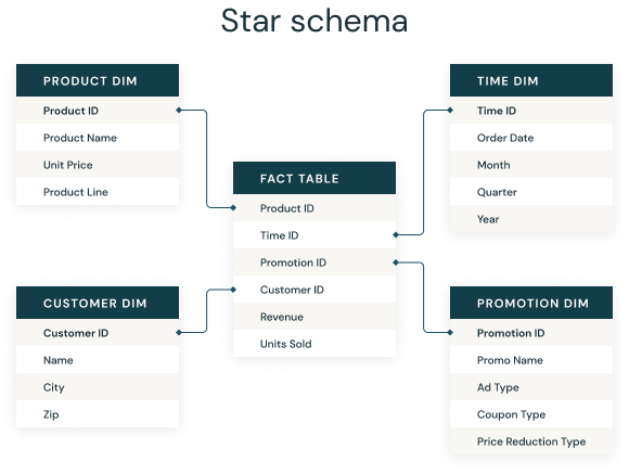
This practice stems from the fact that many information systems take the form of a star schema (@#fig-star-schema-en).
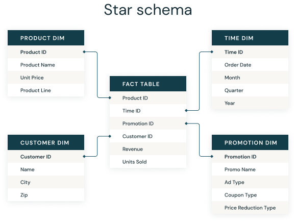
This way of structuring information is closely tied to the relational table model from the 1980s. Today, more flexible data models exist, where information is stored in a data lake without any predefined structure. Nevertheless, the star schema model remains relevant because it makes it possible to organize information around statistical units of interest (the customer, the company, the transaction, etc.) while still allowing data to be compartmentalized.
Since the logic of the star schema historically comes from relational databases, it is natural that it is an approach intrinsically linked to the philosophy of SQL, even in the vocabulary. The term “data join” is often used, inherited from the SQL JOIN term, and the way to describe joins (left join, right join…) comes directly from the associated SQL instructions.
3.2 Joining keys
We refer to join keys as the variable(s) necessary for merging data. These are the variables common to both datasets. They do not need to have the same name, but they must share common values; otherwise, the intersection between these two datasets is the empty set.
We can manipulate two dimensions in the join (this will be clearer later with graphical examples):
- There are mainly three types of merges: left join, right join, or a combination of the two, depending on the type of pivot we want to implement.
- Then, there are two ways to merge the values once we have chosen a pivot: inner or outer join. In the first case, we only keep the observations where the join keys are present in both datasets; in the second, we keep all observations of the pivot key variables, even if the second dataset does not have such observations, resulting in missing values.
In the examples below, we will use the commune codes and departments as join keys. Using the department is not necessary since it is directly deduced from the commune code, but it helps illustrate the principle of joins on multiple variables. Note that the name of the commune is intentionally set aside for joins, even though it is common information to both datasets. However, as it is a textual field, which may follow different formatting norms in the two datasets, it is not reliable for an exact join.
To illustrate the principle of the left or right pivot, we will create two identifier variables for the row in our left and right datasets. This will allow us to easily find rows present in one dataset but not in the other.
emissions = emissions.reset_index(names = ['id_left'])
filosofi = filosofi.reset_index(names = ['id_right'])
4 Implementation with Pandas
In Pandas, the most practical method to join datasets based on common characteristics is merge. Its main arguments allow for controlling the join behavior. We will explore them visually.
In our case, for constructing statistics on carbon emissions, the left base will be the emissions DataFrame, and the right base will be the filosofi DataFrame:
emissions.head(2)| id_left | INSEE commune | Commune | Agriculture | Autres transports | Autres transports international | CO2 biomasse hors-total | Déchets | Energie | Industrie hors-énergie | Résidentiel | Routier | Tertiaire | dep | |
|---|---|---|---|---|---|---|---|---|---|---|---|---|---|---|
| 0 | 0 | 01001 | L'ABERGEMENT-CLEMENCIAT | 3711.425991 | NaN | NaN | 432.751835 | 101.430476 | 2.354558 | 6.911213 | 309.358195 | 793.156501 | 367.036172 | 01 |
| 1 | 1 | 01002 | L'ABERGEMENT-DE-VAREY | 475.330205 | NaN | NaN | 140.741660 | 140.675439 | 2.354558 | 6.911213 | 104.866444 | 348.997893 | 112.934207 | 01 |
filosofi.head(2)| id_right | CODGEO | LIBGEO | POPULATION | NIVVIE_MEDIAN | TAUX_PAUVRETE | dep | |
|---|---|---|---|---|---|---|---|
| 0 | 0 | 01001 | L'Abergement-Clémenciat | 860 | 28270.0 | NaN | 01 |
| 1 | 1 | 01002 | L'Abergement-de-Varey | 270 | 28140.0 | NaN | 01 |
4.1 Left join
Let’s start with the left join. As its name indicates, we will take the left variable as the pivot:
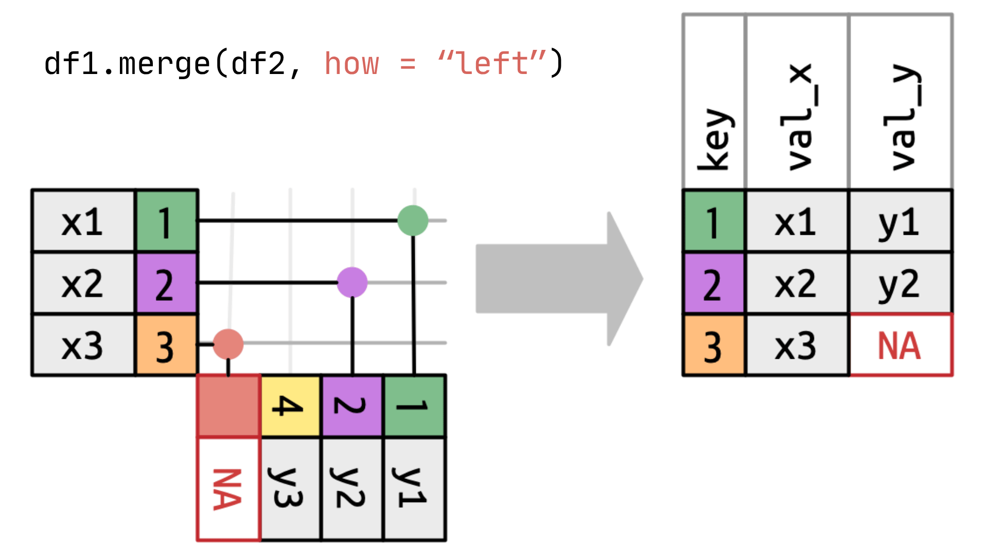
left_merged = emissions.merge(
  filosofi,
  left_on = ["INSEE commune", "dep"],
  right_on = ["CODGEO", "dep"],
  how = "left"
)
left_merged.head(3)| id_left | INSEE commune | Commune | Agriculture | Autres transports | Autres transports international | CO2 biomasse hors-total | Déchets | Energie | Industrie hors-énergie | Résidentiel | Routier | Tertiaire | dep | id_right | CODGEO | LIBGEO | POPULATION | NIVVIE_MEDIAN | TAUX_PAUVRETE | |
|---|---|---|---|---|---|---|---|---|---|---|---|---|---|---|---|---|---|---|---|---|
| 0 | 0 | 01001 | L'ABERGEMENT-CLEMENCIAT | 3711.425991 | NaN | NaN | 432.751835 | 101.430476 | 2.354558 | 6.911213 | 309.358195 | 793.156501 | 367.036172 | 01 | 0.0 | 01001 | L'Abergement-Clémenciat | 860.0 | 28270.0 | NaN |
| 1 | 1 | 01002 | L'ABERGEMENT-DE-VAREY | 475.330205 | NaN | NaN | 140.741660 | 140.675439 | 2.354558 | 6.911213 | 104.866444 | 348.997893 | 112.934207 | 01 | 1.0 | 01002 | L'Abergement-de-Varey | 270.0 | 28140.0 | NaN |
| 2 | 2 | 01004 | AMBERIEU-EN-BUGEY | 499.043526 | 212.577908 | NaN | 10313.446515 | 5314.314445 | 998.332482 | 2930.354461 | 16616.822534 | 15642.420313 | 10732.376934 | 01 | 2.0 | 01004 | Ambérieu-en-Bugey | 15934.0 | 24210.0 | 18.0 |
It is recommended to always explicitly specify the join keys using the left_on, right_on, or on arguments if the variable names are common between the two datasets.
If there are common variable names between the datasets that are not defined as join keys, they will not be used for the join but will be retained with a suffix that defaults to _x and _y (configurable using the suffixes argument).
The Pandas syntax is directly inspired by SQL, so we have a fairly transparent translation of the above instruction into SQL:
SELECT *
FROM emissions
LEFT JOIN filosofi
  ON emissions.`INSEE commune` = filosofi.CODGEO
  AND emissions.dep = filosofi.dep;
By performing a left join, we should, in principle, have as many rows as in the left dataset:
left_merged.shape[0] == emissions.shape[0]TrueOtherwise, it indicates that there is a duplicate key on the right. Thanks to our id_right variable, we can identify the commune codes on the right that do not exist on the left:
left_merged.loc[left_merged['id_right'].isna()].tail(3)| id_left | INSEE commune | Commune | Agriculture | Autres transports | Autres transports international | CO2 biomasse hors-total | Déchets | Energie | Industrie hors-énergie | Résidentiel | Routier | Tertiaire | dep | id_right | CODGEO | LIBGEO | POPULATION | NIVVIE_MEDIAN | TAUX_PAUVRETE | |
|---|---|---|---|---|---|---|---|---|---|---|---|---|---|---|---|---|---|---|---|---|
| 35552 | 35552 | 93059 | PIERREFITTE-SUR-SEINE | 3.384360 | 293.997505 | NaN | 8462.785892 | 63344.922645 | 915.922961 | 2688.461993 | 22146.952752 | 24167.708776 | 14417.152611 | 93 | NaN | NaN | NaN | NaN | NaN | NaN |
| 35687 | 35687 | 95259 | GADANCOURT | 312.298700 | NaN | NaN | 142.113291 | 11.372909 | NaN | NaN | 32.440647 | 2060.981036 | 41.153991 | 95 | NaN | NaN | NaN | NaN | NaN | NaN |
| 35693 | 35693 | 95282 | GOUZANGREZ | 826.234401 | NaN | NaN | 53.146172 | 23.274790 | 2.354558 | 6.911213 | 55.638159 | 36.040818 | 84.222120 | 95 | NaN | NaN | NaN | NaN | NaN | NaN |
This is because the two datasets do not rely on the same version of the official geographical code. The Filosofi data, disseminated via the Melodi API, reflects the most recent municipal boundaries (2025), whereas the Ademe emissions data, although updated in 2025, has not yet caught up with some recent commune mergers. For example, the commune of Courcouronnes is still present as such in the emissions data (left base):
left_merged.loc[
  left_merged['id_right'].isna()
  & left_merged['Commune'].str.contains("COURCOURONNES", na=False)
]| id_left | INSEE commune | Commune | Agriculture | Autres transports | Autres transports international | CO2 biomasse hors-total | Déchets | Energie | Industrie hors-énergie | Résidentiel | Routier | Tertiaire | dep | id_right | CODGEO | LIBGEO | POPULATION | NIVVIE_MEDIAN | TAUX_PAUVRETE | |
|---|---|---|---|---|---|---|---|---|---|---|---|---|---|---|---|---|---|---|---|---|
| 35348 | 35348 | 91182 | COURCOURONNES | 24.548795 | 103.360309 | NaN | 9623.065698 | 111.241872 | 1276.170296 | 3745.877636 | 9978.002088 | 57834.224552 | 10532.120761 | 91 | NaN | NaN | NaN | NaN | NaN | NaN |
Yet this commune has since merged with Evry to form the new commune of Évry-Courcouronnes, the only form under which it now appears in the Filosofi data (right base):
filosofi.loc[
  filosofi['LIBGEO']
  .str.lower()
  .str.contains("courcouronnes", na=False)
]| id_right | CODGEO | LIBGEO | POPULATION | NIVVIE_MEDIAN | TAUX_PAUVRETE | dep | |
|---|---|---|---|---|---|---|---|
| 34315 | 34315 | 91228 | Évry-Courcouronnes | 66919 | 21020.0 | 28.6 | 91 |
In a public statistics construction exercise, we could not afford this discrepancy in years.
4.2 Right join
The principle is the same, but this time it is the right base that is taken as the pivot:
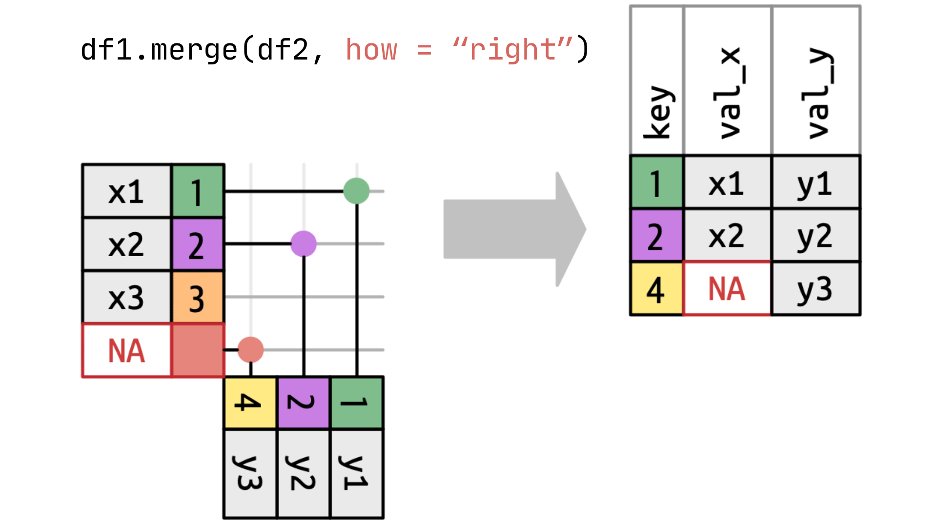
right_merged = emissions.merge(
  filosofi,
  left_on = ["INSEE commune", "dep"],
  right_on = ["CODGEO", "dep"],
  how = "right"
)
right_merged.head(3)| id_left | INSEE commune | Commune | Agriculture | Autres transports | Autres transports international | CO2 biomasse hors-total | Déchets | Energie | Industrie hors-énergie | Résidentiel | Routier | Tertiaire | dep | id_right | CODGEO | LIBGEO | POPULATION | NIVVIE_MEDIAN | TAUX_PAUVRETE | |
|---|---|---|---|---|---|---|---|---|---|---|---|---|---|---|---|---|---|---|---|---|
| 0 | 0.0 | 01001 | L'ABERGEMENT-CLEMENCIAT | 3711.425991 | NaN | NaN | 432.751835 | 101.430476 | 2.354558 | 6.911213 | 309.358195 | 793.156501 | 367.036172 | 01 | 0 | 01001 | L'Abergement-Clémenciat | 860 | 28270.0 | NaN |
| 1 | 1.0 | 01002 | L'ABERGEMENT-DE-VAREY | 475.330205 | NaN | NaN | 140.741660 | 140.675439 | 2.354558 | 6.911213 | 104.866444 | 348.997893 | 112.934207 | 01 | 1 | 01002 | L'Abergement-de-Varey | 270 | 28140.0 | NaN |
| 2 | 2.0 | 01004 | AMBERIEU-EN-BUGEY | 499.043526 | 212.577908 | NaN | 10313.446515 | 5314.314445 | 998.332482 | 2930.354461 | 16616.822534 | 15642.420313 | 10732.376934 | 01 | 2 | 01004 | Ambérieu-en-Bugey | 15934 | 24210.0 | 18.0 |
The equivalent instruction in SQL would be:
SELECT *
FROM filosofi
RIGHT JOIN emissions
  ON filosofi.CODGEO = emissions.`INSEE commune`
  AND filosofi.dep = emissions.dep;
We can, as before, check the consistency of the dimensions:
right_merged.shape[0] == filosofi.shape[0]TrueTo check the number of rows in the Filosofi data that we do not have in our greenhouse gas emissions dataset, we can do:
right_merged['id_left'].isna().sum()np.int64(120)It’s a small number. What are these observations?
right_merged.loc[
  right_merged['id_left'].isna(),
  filosofi.columns.tolist() + emissions.columns.tolist()
]| id_right | CODGEO | LIBGEO | POPULATION | NIVVIE_MEDIAN | TAUX_PAUVRETE | dep | id_left | INSEE commune | Commune | ... | Autres transports | Autres transports international | CO2 biomasse hors-total | Déchets | Energie | Industrie hors-énergie | Résidentiel | Routier | Tertiaire | dep | |
|---|---|---|---|---|---|---|---|---|---|---|---|---|---|---|---|---|---|---|---|---|---|
| 4201 | 4201 | 12218 | NaN | 1540 | 24390.0 | NaN | 12 | NaN | NaN | NaN | ... | NaN | NaN | NaN | NaN | NaN | NaN | NaN | NaN | NaN | 12 |
| 4338 | 4338 | 13055 | Marseille | 886040 | 22860.0 | 28.1 | 13 | NaN | NaN | NaN | ... | NaN | NaN | NaN | NaN | NaN | NaN | NaN | NaN | NaN | 13 |
| 17537 | 17537 | 49126 | NaN | 17162 | 25770.0 | 7.0 | 49 | NaN | NaN | NaN | ... | NaN | NaN | NaN | NaN | NaN | NaN | NaN | NaN | NaN | 49 |
| 27039 | 27039 | 69123 | Lyon | 519127 | 28290.0 | 18.0 | 69 | NaN | NaN | NaN | ... | NaN | NaN | NaN | NaN | NaN | NaN | NaN | NaN | NaN | 69 |
| 29194 | 29194 | 75056 | Paris | 2103778 | 33650.0 | 16.8 | 75 | NaN | NaN | NaN | ... | NaN | NaN | NaN | NaN | NaN | NaN | NaN | NaN | NaN | 75 |
| ... | ... | ... | ... | ... | ... | ... | ... | ... | ... | ... | ... | ... | ... | ... | ... | ... | ... | ... | ... | ... | ... |
| 34853 | 34853 | 97420 | Sainte-Suzanne | 25551 | 19560.0 | 34.9 | 97 | NaN | NaN | NaN | ... | NaN | NaN | NaN | NaN | NaN | NaN | NaN | NaN | NaN | 97 |
| 34854 | 34854 | 97421 | Salazie | 7268 | 15180.0 | 53.0 | 97 | NaN | NaN | NaN | ... | NaN | NaN | NaN | NaN | NaN | NaN | NaN | NaN | NaN | 97 |
| 34855 | 34855 | 97422 | Le Tampon | 82579 | 18470.0 | 38.1 | 97 | NaN | NaN | NaN | ... | NaN | NaN | NaN | NaN | NaN | NaN | NaN | NaN | NaN | 97 |
| 34856 | 34856 | 97423 | Les Trois-Bassins | 7221 | 18980.0 | 35.0 | 97 | NaN | NaN | NaN | ... | NaN | NaN | NaN | NaN | NaN | NaN | NaN | NaN | NaN | 97 |
| 34857 | 34857 | 97424 | Cilaos | 5040 | 15660.0 | 49.0 | 97 | NaN | NaN | NaN | ... | NaN | NaN | NaN | NaN | NaN | NaN | NaN | NaN | NaN | 97 |
120 rows × 21 columns
It is surprising to see that Paris, Lyon, and Marseille are present in the communal statistics dataset but not in the emissions dataset. To understand why, let’s search in our emissions data for observations related to Marseille:
emissions.loc[
  emissions["Commune"]
  .str.upper()
  .str.contains('MARSEILLE-')
]| id_left | INSEE commune | Commune | Agriculture | Autres transports | Autres transports international | CO2 biomasse hors-total | Déchets | Energie | Industrie hors-énergie | Résidentiel | Routier | Tertiaire | dep | |
|---|---|---|---|---|---|---|---|---|---|---|---|---|---|---|
| 4462 | 4462 | 13201 | MARSEILLE-1ER-ARRONDISSEMENT | 303.836964 | 850.796099 | NaN | 18749.902852 | 2572.980666 | 2366.477690 | 6946.201368 | 29755.542456 | 35324.129125 | 18535.087435 | 13 |
| 4463 | 4463 | 13202 | MARSEILLE-2E-ARRONDISSEMENT | 303.836964 | 83.384844 | NaN | 14248.781083 | 2451.230873 | 2366.477690 | 6946.201368 | 18629.702329 | 35324.129125 | 11530.097205 | 13 |
| 4464 | 4464 | 13203 | MARSEILLE-3E-ARRONDISSEMENT | 303.836964 | 18.238987 | NaN | 20705.839485 | 2627.535940 | 2366.477690 | 6946.201368 | 32283.391803 | 35324.129125 | 21695.331089 | 13 |
| 4465 | 4465 | 13204 | MARSEILLE-4E-ARRONDISSEMENT | 303.836964 | 84.063314 | NaN | 21525.141519 | 2649.386137 | 2366.477690 | 107849.501368 | 34633.530963 | 35324.129125 | 22961.055568 | 13 |
| 4466 | 4466 | 13205 | MARSEILLE-5E-ARRONDISSEMENT | 303.836964 | NaN | NaN | 21220.562849 | 2641.273890 | 2366.477690 | 6946.201368 | 46460.016400 | 35324.129125 | 22498.466001 | 13 |
| 4467 | 4467 | 13206 | MARSEILLE-6E-ARRONDISSEMENT | 303.836964 | NaN | NaN | 19817.462943 | 2602.050928 | 2366.477690 | 6946.201368 | 32135.350914 | 35324.129125 | 20219.051308 | 13 |
| 4468 | 4468 | 13207 | MARSEILLE-7E-ARRONDISSEMENT | 303.836964 | NaN | NaN | 17667.589643 | 2544.306929 | 2366.477690 | 6946.201368 | 26082.234669 | 35324.129125 | 17252.687971 | 13 |
| 4469 | 4469 | 13208 | MARSEILLE-8E-ARRONDISSEMENT | 303.836964 | NaN | NaN | 31033.598562 | 2905.706707 | 2366.477690 | 6946.201368 | 46457.720220 | 35324.129125 | 38019.611886 | 13 |
| 4470 | 4470 | 13209 | MARSEILLE-9E-ARRONDISSEMENT | 303.836964 | 206.323957 | 15168.902916 | 63507.303272 | 2866.252439 | 2366.477690 | 6946.201368 | 53791.270123 | 35324.129125 | 41201.045974 | 13 |
| 4471 | 4471 | 13210 | MARSEILLE-10E-ARRONDISSEMENT | 303.836964 | NaN | NaN | 23774.329289 | 2709.963639 | 2366.477690 | 6946.201368 | 39770.211148 | 35324.129125 | 27865.799133 | 13 |
| 4472 | 4472 | 13211 | MARSEILLE-11E-ARRONDISSEMENT | 303.836964 | 149.788396 | NaN | 24246.711719 | 2720.116339 | 2366.477690 | 11159.128368 | 41737.276404 | 35324.129125 | 32805.823144 | 13 |
| 4473 | 4473 | 13212 | MARSEILLE-12E-ARRONDISSEMENT | 303.836964 | 34.728224 | NaN | 25332.342243 | 2752.276194 | 2366.477690 | 6946.201368 | 44144.355145 | 35324.129125 | 28921.206190 | 13 |
| 4474 | 4474 | 13213 | MARSEILLE-13E-ARRONDISSEMENT | 303.836964 | NaN | NaN | 34480.339077 | 3001.079306 | 2366.477690 | 6946.201368 | 64717.674768 | 35324.129125 | 43333.716539 | 13 |
| 4475 | 4475 | 13214 | MARSEILLE-14E-ARRONDISSEMENT | 303.836964 | 250.117946 | NaN | 25588.294079 | 2758.463641 | 2366.477690 | 6946.201368 | 43612.783924 | 35324.129125 | 32142.611435 | 13 |
| 4476 | 4476 | 13215 | MARSEILLE-15E-ARRONDISSEMENT | 303.836964 | 320.003252 | NaN | 31565.381887 | 2919.403353 | 2366.477690 | 6946.201368 | 57187.164876 | 35324.129125 | 44748.956297 | 13 |
| 4477 | 4477 | 13216 | MARSEILLE-16E-ARRONDISSEMENT | 303.836964 | 518.266268 | 12.311853 | 12119.260477 | 2392.479039 | 2366.477690 | 20211.201368 | 12795.918860 | 35324.129125 | 10336.618838 | 13 |
| 23522 | 23522 | 60387 | MARSEILLE-EN-BEAUVAISIS | 330.191658 | 90.910961 | NaN | 1430.605647 | 191.355801 | 127.146118 | 373.205521 | 573.997868 | 2780.093648 | 692.439819 | 60 |
This is because the Ademe emissions dataset provides information on districts in the three largest cities, whereas the Insee dataset does not have this breakdown.
4.3 Inner join
This is the dataset where the keys are found at the intersection of the two tables.
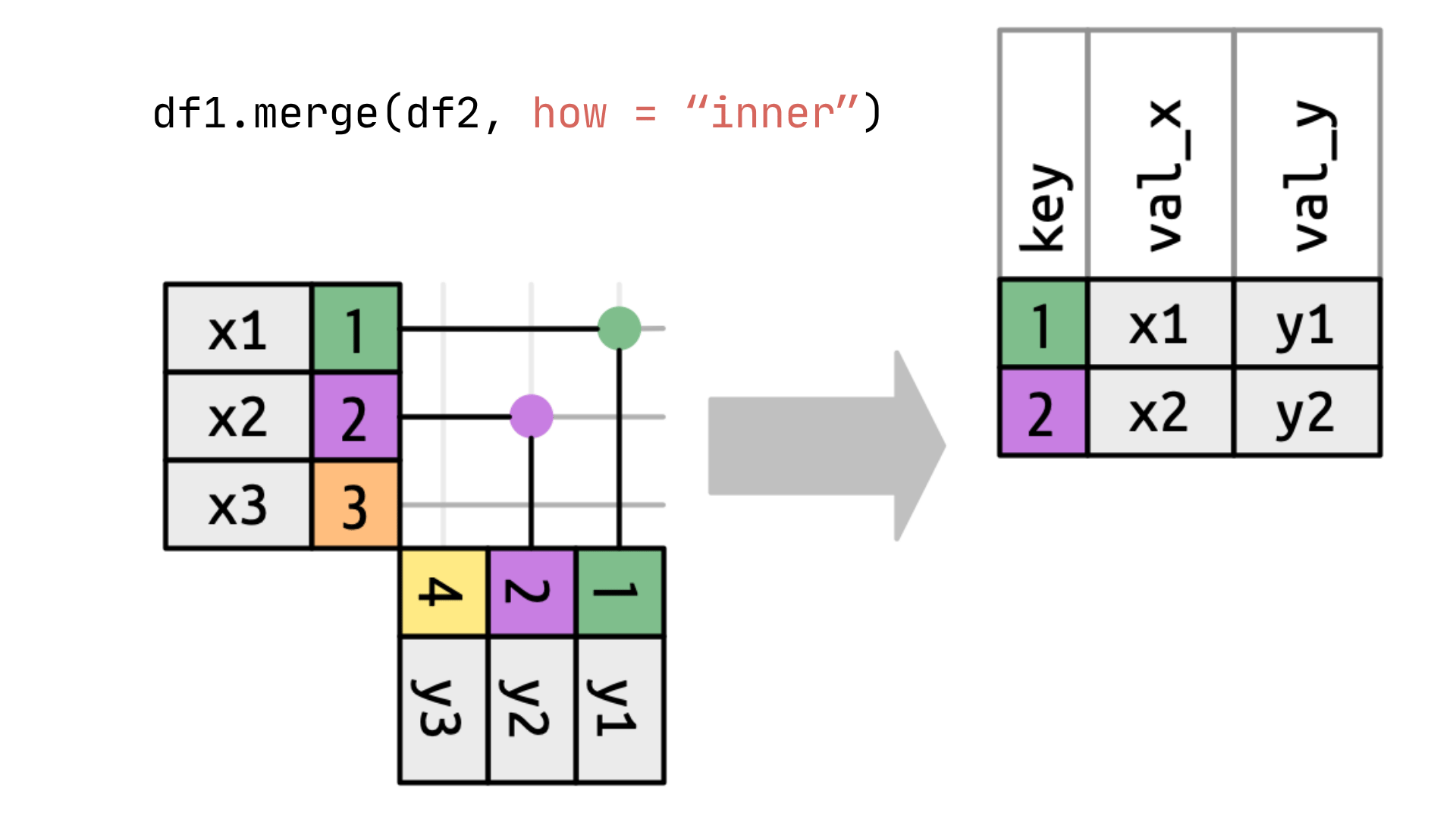
inner_merged = emissions.merge(
  filosofi,
  left_on = ["INSEE commune", "dep"],
  right_on = ["CODGEO", "dep"],
  how = "inner"
)
inner_merged.head(3)| id_left | INSEE commune | Commune | Agriculture | Autres transports | Autres transports international | CO2 biomasse hors-total | Déchets | Energie | Industrie hors-énergie | Résidentiel | Routier | Tertiaire | dep | id_right | CODGEO | LIBGEO | POPULATION | NIVVIE_MEDIAN | TAUX_PAUVRETE | |
|---|---|---|---|---|---|---|---|---|---|---|---|---|---|---|---|---|---|---|---|---|
| 0 | 0 | 01001 | L'ABERGEMENT-CLEMENCIAT | 3711.425991 | NaN | NaN | 432.751835 | 101.430476 | 2.354558 | 6.911213 | 309.358195 | 793.156501 | 367.036172 | 01 | 0 | 01001 | L'Abergement-Clémenciat | 860 | 28270.0 | NaN |
| 1 | 1 | 01002 | L'ABERGEMENT-DE-VAREY | 475.330205 | NaN | NaN | 140.741660 | 140.675439 | 2.354558 | 6.911213 | 104.866444 | 348.997893 | 112.934207 | 01 | 1 | 01002 | L'Abergement-de-Varey | 270 | 28140.0 | NaN |
| 2 | 2 | 01004 | AMBERIEU-EN-BUGEY | 499.043526 | 212.577908 | NaN | 10313.446515 | 5314.314445 | 998.332482 | 2930.354461 | 16616.822534 | 15642.420313 | 10732.376934 | 01 | 2 | 01004 | Ambérieu-en-Bugey | 15934 | 24210.0 | 18.0 |
In SQL, this would be:
SELECT *
FROM emissions
INNER JOIN filosofi
  ON emissions.`INSEE commune` = filosofi.CODGEO
  AND emissions.dep = filosofi.dep;
The number of rows in our dataset can be compared to the left and right datasets:
inner_merged.shape[0] == (
  left_merged.shape[0] - left_merged['id_right'].isna().sum()
)np.True_inner_merged.shape[0] == (
right_merged.shape[0] - right_merged['id_left'].isna().sum()
)np.True_4.4 Full join
The full join is a pivot to the left and then to the right for the information that was not found.
full_merged = emissions.merge(
  filosofi,
  left_on = ["INSEE commune", "dep"],
  right_on = ["CODGEO", "dep"],
  how = "outer"
)
full_merged.head(3)| id_left | INSEE commune | Commune | Agriculture | Autres transports | Autres transports international | CO2 biomasse hors-total | Déchets | Energie | Industrie hors-énergie | Résidentiel | Routier | Tertiaire | dep | id_right | CODGEO | LIBGEO | POPULATION | NIVVIE_MEDIAN | TAUX_PAUVRETE | |
|---|---|---|---|---|---|---|---|---|---|---|---|---|---|---|---|---|---|---|---|---|
| 0 | 0.0 | 01001 | L'ABERGEMENT-CLEMENCIAT | 3711.425991 | NaN | NaN | 432.751835 | 101.430476 | 2.354558 | 6.911213 | 309.358195 | 793.156501 | 367.036172 | 01 | 0.0 | 01001 | L'Abergement-Clémenciat | 860.0 | 28270.0 | NaN |
| 1 | 1.0 | 01002 | L'ABERGEMENT-DE-VAREY | 475.330205 | NaN | NaN | 140.741660 | 140.675439 | 2.354558 | 6.911213 | 104.866444 | 348.997893 | 112.934207 | 01 | 1.0 | 01002 | L'Abergement-de-Varey | 270.0 | 28140.0 | NaN |
| 2 | 2.0 | 01004 | AMBERIEU-EN-BUGEY | 499.043526 | 212.577908 | NaN | 10313.446515 | 5314.314445 | 998.332482 | 2930.354461 | 16616.822534 | 15642.420313 | 10732.376934 | 01 | 2.0 | 01004 | Ambérieu-en-Bugey | 15934.0 | 24210.0 | 18.0 |
As usual, the translation to SQL is almost immediate:
SELECT *
FROM emissions
FULL OUTER JOIN filosofi
  ON emissions.`INSEE commune` = filosofi.CODGEO
  AND emissions.dep = filosofi.dep;
This time, we have a combination of our three initial datasets:
- The inner join;
- The left join on observations without the right key;
- The right join on observations without the left key;
(
  full_merged['id_left'].isna().sum() + full_merged['id_right'].isna().sum()
) == (
  left_merged['id_right'].isna().sum() + right_merged['id_left'].isna().sum()
)np.True_The id_left and id_right columns were only useful to illustrate the joins above. We drop them from our datasets before moving on, so they do not interfere with later processing:
emissions = emissions.drop(columns = ['id_left'])
filosofi = filosofi.drop(columns = ['id_right'])
4.5 In summary
The four main types of join are the following
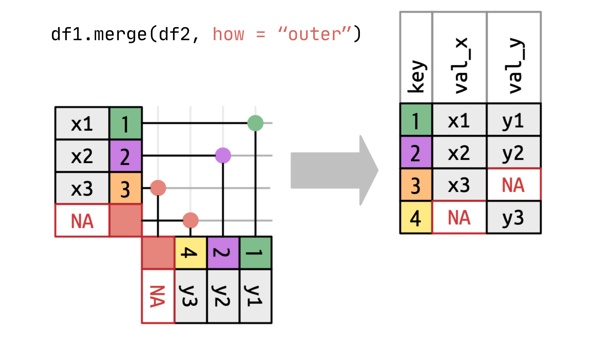
Main database join methods
In a funny representation, this gives:

There are of course other types of joins, based on negation: semi-join, anti-join, etc. These methods are less frequently used but are useful when trying to determine the discrepancy between two datasets.
5 Examples of identifiers in French data
We have highlighted the value of having identifiers common to several databases rather than relying on noisy textual information. We will now discuss three identifiers that matter to users of French data:
- The official geographic code, a unique identifier for geographic data
- The NIR, or social security number, the French individual identifier
- The SIRENE code, a unique identifier for businesses operating in France.
5.1 The Official Geographic Code (COG): The identifier for geographic data
For geographic data, there are many identifiers depending on the study problem.
Among the main needs is the ability to match geographic data using a common administrative identifier. For example, associating two datasets at the municipal level.
For this, the reference identifier is the Insee code, derived from the Official Geographic Code (COG), which we have been using since the last chapter and will extensively use throughout the different chapters of this course. Given that the administrative geography is constantly evolving, the Insee code database is a living base. The Insee website and APIs provide access to the post-war historical data for long-term geographic analysis.
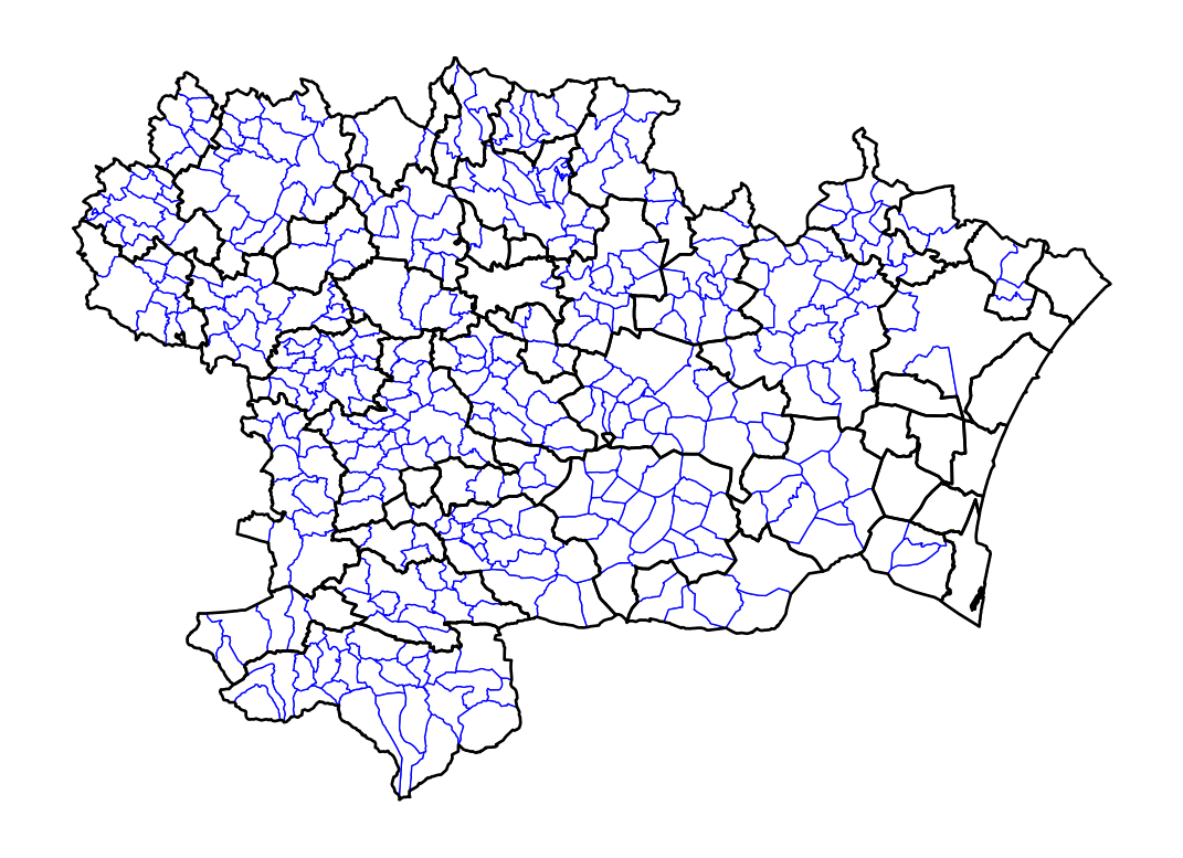
Postal codes cannot be considered as an identifier: they can group several municipalities or, conversely, one municipality can have several postal codes. It is a system managed by La Poste that was not designed for statistical analysis.
To illustrate the problem, from the data provided by La Poste, we can see that postal code 11420 corresponds to 11 municipalities:
codes_postaux = pd.read_csv(
  "https://datanova.laposte.fr/data-fair/api/v1/datasets/laposte-hexasmal/raw",
  sep = ";", encoding = "latin1",
  dtype = {"Code_postal": "str", "#Code_commune_INSEE": "str"}
)
codes_postaux.loc[codes_postaux['Code_postal'] == "11420"]| #Code_commune_INSEE | Nom_de_la_commune | Code_postal | Libellé_d_acheminement | Ligne_5 | |
|---|---|---|---|---|---|
| 3921 | 11033 | BELPECH | 11420 | BELPECH | NaN |
| 3944 | 11057 | CAHUZAC | 11420 | CAHUZAC | NaN |
| 4080 | 11184 | LAFAGE | 11420 | LAFAGE | NaN |
| 4124 | 11226 | MAYREVILLE | 11420 | MAYREVILLE | NaN |
| 4134 | 11236 | MOLANDIER | 11420 | MOLANDIER | NaN |
| 4176 | 11277 | PECHARIC ET LE PY | 11420 | PECHARIC ET LE PY | NaN |
| 4177 | 11278 | PECH LUNA | 11420 | PECH LUNA | NaN |
| 4182 | 11283 | PEYREFITTE SUR L HERS | 11420 | PEYREFITTE SUR L HERS | NaN |
| 4189 | 11290 | PLAIGNE | 11420 | PLAIGNE | NaN |
| 4264 | 11365 | ST SERNIN | 11420 | ST SERNIN | NaN |
| 4317 | 11419 | VILLAUTOU | 11420 | VILLAUTOU | NaN |
Anticipating on the skills developed in the upcoming chapters, we can represent the problem cartographically by taking the example of the Aude department. The code to produce the map of commune codes is given as is, not developed, as it uses concepts and libraries that will be presented in the next chapter:
from cartiflette import carti_download

shp_communes = carti_download(
  values = ["11"],
  crs = 4326,
  borders = "COMMUNE",
  simplification=50,
  filter_by="DEPARTEMENT",
  source="EXPRESS-COG-CARTO-TERRITOIRE",
1  year=2022)

codes_postaux11 = shp_communes.merge(
  codes_postaux,
  left_on = "INSEE_COM",
  right_on = "#Code_commune_INSEE"
2)
3codes_postaux11 = codes_postaux11.dissolve(by = "Code_postal")- 1
-
Downloading the official contours of Aude produced by IGN using the
cartiflettelibrary - 2
- Joining using the commune code between the two data sources
- 3
- Aggregating the geometry at the postal code level
1# Map
ax = shp_communes.plot(color='white', edgecolor='blue', linewidth = 0.5)
ax = codes_postaux11.plot(ax = ax, color='none', edgecolor='black')
ax.set_axis_off()- 1
- Creating a map from our two layers
5.1.1 Sirene: the identifier in business data
To connect French business microdata, there is a unique identification number: the Siren number. It is an identification number in a legal business directory essential for all legal, fiscal, and other procedures. For companies that have multiple establishments—for example, in several cities—there is a derived identifier called the Siret: the 9 digits of the Siren number are followed by 5 establishment identification digits. Moreover, public administrations are also concerned with the Siren number: being involved in market operations (purchasing equipment, renting goods, etc.), they also have a Siren identifier. As they are registered in legal directories whose information is public, the Siren numbers and the associated company names are available in open data, for example, on annuaire-entreprises.data.gouv.fr/ for occasional searches, or on data.gouv.fr.
This Sirene database is a treasure trove of information, sometimes amusing, about French companies. For example, the site tif.hair/ cataloged the proportion of hair salons with puns in their names. When an entrepreneur declares the creation of a business, they receive a Siren number and an activity code (the APE code) related to the description of their business activity. This code allows the classification of a business activity in the French Classification of Activities (NAF), which will be used by Insee for the publication of sectoral statistics. In the case of hairdressers, the code in the NAF is 96.02A. From the open data available, it is possible, in a few lines of Python, to get the list of all hairdressers and then explore this data (the subject of the next optional exercise).
The following optional exercise suggests replicating, in a simplified manner, the survey done by tif.hair/ on puns in hair salon names. It allows practicing some text manipulation methods, ahead of the chapter dedicated to regular expressions.
Since the dataset of all companies is quite large (around 4GB in CSV after decompression), it is more practical to use a dataset in Parquet format, which is more optimized (more details on this format in the advanced chapter dedicated to it).
To read this type of file optimally, it is recommended to use the DuckDB library, which allows consuming only the necessary data instead of downloading the entire file to read only a part of it as would be the case with Pandas (see the last chapter of this part, section “Beyond Pandas”). The following SQL query translates into natural language as: “From the Parquet file, I only want a few columns of the file for hairdressers (APE: 96.02A) whose business name (denominationUsuelleEtablissement) is provided”:
import duckdb
coiffeurs = duckdb.sql("""
  SELECT
    siren, siret, dateDebut, enseigne1Etablissement, activitePrincipaleEtablissement, denominationUsuelleEtablissement
  FROM
    read_parquet('https://minio.lab.sspcloud.fr/lgaliana/data/sirene2024.parquet')
  WHERE
    activitePrincipaleEtablissement == '96.02A'
    AND
    denominationUsuelleEtablissement IS NOT NULL
""")
1coiffeurs = coiffeurs.df()- 1
- Convert the DuckDB dataframe to a Pandas DataFrame.
coiffeurs.head(3)| siren | siret | dateDebut | enseigne1Etablissement | activitePrincipaleEtablissement | denominationUsuelleEtablissement | |
|---|---|---|---|---|---|---|
| 0 | 024050379 | 02405037900023 | 2016-01-14 | NaN | 96.02A | SOPHA COIFFURE |
| 1 | 024076481 | 02407648100019 | 2017-07-17 | NaN | 96.02A | SAF COIFFURE |
| 2 | 047142872 | 04714287200036 | 2011-07-31 | NaN | 96.02A | JENNY |
TipOptional Exercise: Punny Hairdressers
In this exercise, we will consider only the variable denominationUsuelleEtablissement.
- In this dataset,
[ND]is a code for missing value. SincePythonhas no reason to know this a priori and therefore didn’t interpret these values as missing, use thereplacemethod to replace[ND]with an empty text field. Also, recode missing values as an empty text field to avoid future errors related to the inability to apply certain text methods to missing values. - Search for all occurrences where the term
tifappears, paying attention to the capitalization of the variable. Look at some observations. - Using this example, normalize the names of the salons by removing special characters and count the most frequent puns.
With question 2, we find a list of quite imaginative puns based on the term tif
"IMAGINA'TIF, DIMINUT'TIF, A L'INFINI'TIF, TIF'ANNICK, A TRAC TIF, BLEV HAIR TIF, CHRIS TIF, OBJECTIF PRESTIGE, TIF'ALIZEA HAIRCUT, JS CREA TIF"In a more interactive form, here’s a list of all the hairdressers who have the word tif in the name of their registered business in the official data:
Of course, to go further, it would be better to normalize the data more thoroughly, check that the information sought is not spread across multiple columns, and conduct visual inspections to detect hidden puns. But already, in just a few minutes, we have partial statistics on the phenomenon of punny hairdressers.
5.1.2 The social security number and the issue of individual identifiers’ confidentiality
For individuals, there exists a unique identifier that allows linking them across different data sources: the NIR, also known as the INSEE number or social security number. This number is necessary for the administration to manage social benefits (health, retirement, family…). Beyond this function, which can be useful daily, this number is a unique individual identifier in the National Register of Physical Persons (RNIPP).
This identifier is mainly present in management databases related to payroll, social benefits, etc. However, unlike the Sirene number, it contains several sensitive pieces of information and is inherently linked to the sensitive issue of social security rights.

To address this problem, the non-significant statistical code (CSNS) or hashed NIR, a non-identifying anonymous individual identifier, was recently implemented. The goal of this anonymized identifier is to reduce the dissemination of personal information that, although allowing civil servants and researchers to deterministically link numerous databases, provided analysts with non-essential information about the individuals in question. Bénichou et al. (2023) describe in more detail how French official statistics organizations can use this unique non-significant code to link various data sources with one another.
5.2 Why do we need a commune code when we already have its name?
This exercise will take a step back to understand why we assumed above that the commune code was the key for joining data.
Tip 5.1: Verification of Join Keys
Let’s start by checking the dimensions of the DataFrames and the structure of some key variables.
In this case, the fundamental variables for linking our data are the communal variables.
Here, we have two geographical variables: a commune code and a commune name.
Check the dimensions of the
DataFrames.Identify in
filosofithe commune names that correspond to multiple commune codes and select their codes. In other words, identify theLIBGEOwhere there are duplicateCODGEOand store them in a vectorx(tip: be careful with the index ofx).
We temporarily focus on observations where the label involves more than two different commune codes.
Question 3. Look at these observations in
filosofi.Question 4. To get a better view, reorder the obtained dataset alphabetically.
Question 5. Determine the average size (variable number of people:
POPULATION) and some descriptive statistics of this data. Compare it to the same statistics on the data where labels and commune codes coincide.Question 6. Check the major cities (more than 100,000 people) for the proportion of cities where the same name is associated with different commune codes.
Question 7. Check in
filosofithe cities where the label is equal to Montreuil. Also, check those that contain the term ‘Saint-Denis’.
This small exercise reassures us as the duplicated labels are actually the same commune names but in different departments. So, these are not duplicated observations. We can thus rely on the commune codes, which are unique.
5.3 Associating different sources to compute carbon footprints
Tip 5.2: Calculate the carbon footprint per capita
First, we will calculate the carbon footprint of each commune.
Create a variable
emissionsthat corresponds to the total emissions of a commune.Perform a left join between the emissions data and the framing data[^notebiais].
Calculate the carbon footprint (total emissions / population).
At this stage, we might want to move towards modeling to try to explain the determinants of the carbon footprint based on communal variables. However, for an inferential approach to be relevant, it is necessary to check some descriptive statistics beforehand.
Generate a histogram of the carbon footprint per commune in level and log.
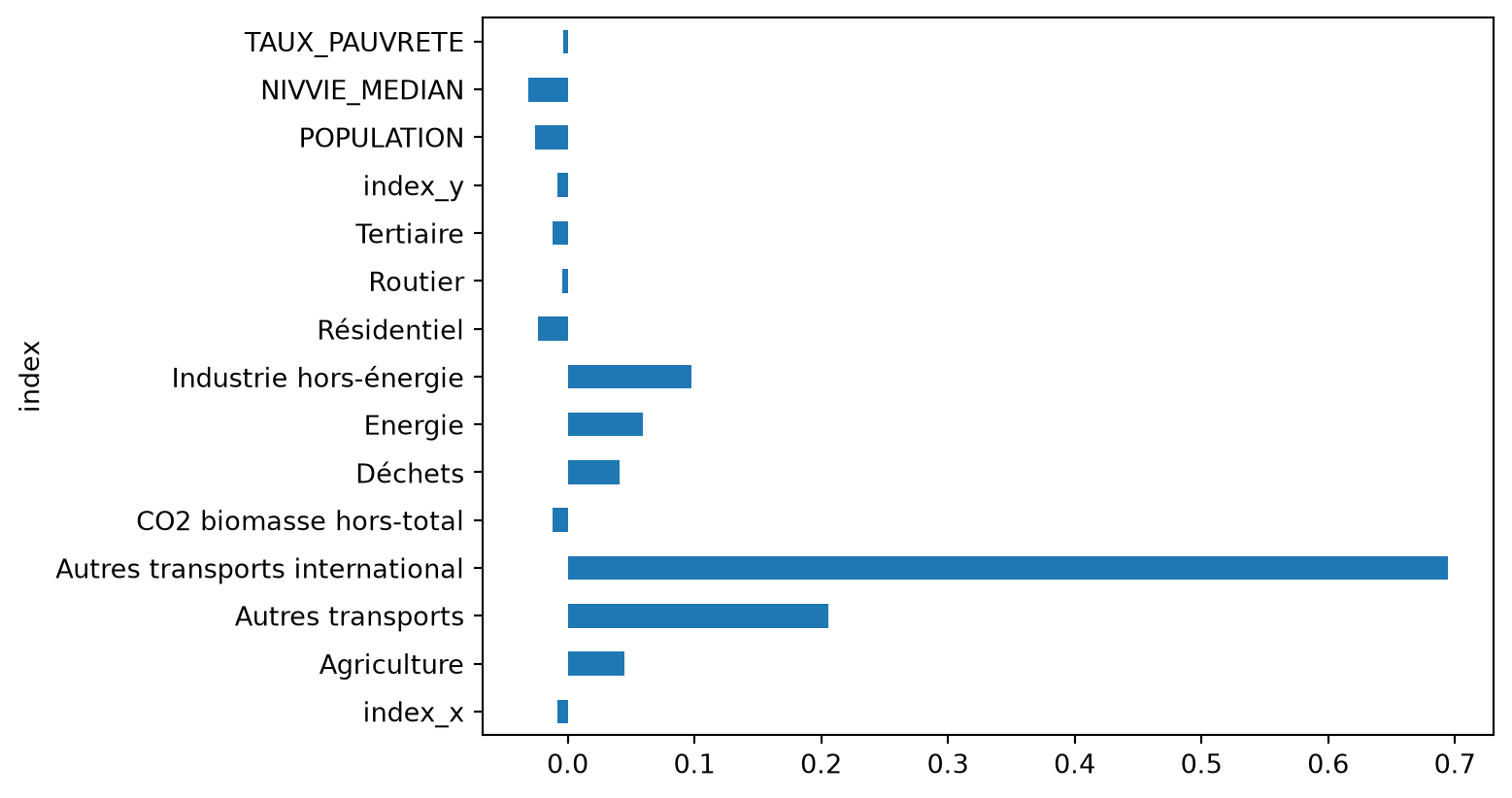
Look at the correlation between the framing variables and the carbon footprint. Do some variables seem to potentially influence the carbon footprint?
At the end of question 5, the correlation graph is as follows:
With a better understanding of our data, gained through this association of sources, we get closer to inferential statistics. In the next chapter, we will continue to use emissions and filosofi, enriched by one another, to build group descriptive statistics and restructure our data.
Informations additionnelles
NotePython environment
This site was built automatically through a Github action using the Quarto
The environment used to obtain the results is reproducible via uv. The pyproject.toml file used to build this environment is available on the linogaliana/python-datascientist repository
pyproject.toml
[project]
name = "python-datascientist"
version = "0.1.0"
description = "Source code for Lino Galiana's Python for data science course"
readme = "README.md"
requires-python = ">=3.13,<3.14"
dependencies = [
    "altair>=6.0.0",
    "cartiflette>=0.2",
    "contextily==1.6.2",
    "duckdb>=0.10.1",
    "folium>=0.19.6",
    "gdal==3.11.4",
    "graphviz==0.20.3",
    "great-tables>=0.12.0",
    "gt-extras>=0.0.8",
    "ipykernel>=6.29.5",
    "jupyter>=1.1.1",
    "jupyter-cache>=1.0.0",
    "kaleido>=0.2.1",
    "langchain-community>=0.3.27",
    "loguru==0.7.3",
    "markdown>=3.8",
    "nbclient>=0.10.0",
    "nbformat>=5.10.4",
    "nltk>=3.9.1",
    "openpyxl>=3.1.5",
    "pandas>=3.0",
    "pip>=25.1.1",
    "plotly>=6.1.2",
    "plotnine>=0.15",
    "polars>=1.8.2",
    "py7zr>=1.1.3",
    "pyarrow>=17.0.0",
    "pynsee>=0.1.8",
    "python-dotenv>=1.0.1",
    "python-frontmatter>=1.1.0",
    "pywaffle>=1.1.1",
    "requests>=2.32.3",
    "scikit-image>=0.24.0",
    "scikit-learn>=1.8.0",
    "scipy>=1.13.0",
    "seaborn>=0.13.2",
    "selenium<4.39.0",
    "spacy>=3.8.4",
    "webdriver-manager>=4.0.2",
    "wordcloud==1.9.3",
]

[tool.uv.sources]
gdal = [
  { index = "gdal-wheels", marker = "sys_platform == 'linux'" },
  { index = "geospatial_wheels", marker = "sys_platform == 'win32'" },
]

[[tool.uv.index]]
name = "geospatial_wheels"
url = "https://nathanjmcdougall.github.io/geospatial-wheels-index/"
explicit = true

[[tool.uv.index]]
name = "gdal-wheels"
url = "https://gitlab.com/api/v4/projects/61637378/packages/pypi/simple"
explicit = true

[dependency-groups]
dev = [
    "nb-clean>=4.0.1",
]
To use exactly the same environment (version of Python and packages), please refer to the documentation for uv.
NoteFile history
References
Bénichou, Yves-Laurent, Lionel Espinasse, and Séverine Gilles. 2023. “Le Code statistique non signifiant (CSNS) : un service pour faciliter les appariements de fichiers.” Courrier des Statistiques, no. 9 (June): 64–85. https://insee.hal.science/hal-05295572.
Wickham, Hadley, Mine Çetinkaya-Rundel, and Garrett Grolemund. 2023. R for Data Science. " O’Reilly Media, Inc."
Footnotes
For demographic data, we directly use the legal populations published by Insee, derived from the census, rather than a fiscal-population proxy. An open exercise is also proposed to construct population aggregates from anonymized individual census data (the detailed files).↩︎
Otherwise, we enter the world of fuzzy matching or probabilistic matching.
Fuzzy matching refers to situations where we no longer have an exact identifier to link two databases, but rather partially noisy information shared between two sources that can be used to establish the connection. For example, a product database might contain
Coca Cola 33CLwhile another containsCoca Cola can, yet both names refer to the same product. Text distance techniques, for instance, can be used to link these observations together. This is typically what a search engine does.Probabilistic matching is another type of approach. Here, observations in two databases are linked not on the basis of an identifier, but on the distance between a set of characteristics across the two databases. This technique is widely used in medical statistics or in public policy evaluation, based on propensity score matching.↩︎
Citation
BibTeX citation:
@book{galiana2025,
  author = {Galiana, Lino},
  title = {Python Pour La Data Science},
  date = {2025},
  url = {https://pythonds.linogaliana.fr/},
  doi = {10.5281/zenodo.8229676},
  langid = {en}
}
For attribution, please cite this work as:
Galiana, Lino. 2025. Python Pour La Data Science. https://doi.org/10.5281/zenodo.8229676.